(1)
| R.J. Allen | R.T. Collis | C. Herold | R.I. Presnell |
| BACK to Section VI Index | | | BACK to Contents Page |
This chapter covers studies of radar capabilities and limitations as they may be related to the apparent manifestation of unidentified flying objects. The studies were carried out by the Stanford Research Institute pursuant to a contract with University of Colorado (Order No. 73403) dated 23 June 1967, under sub-contract to the U.S. Air Force.
The preceding chapter of this report, entitled "Optical Mirage - A Survey of the Literature," by William Viezee, covers optical phenomena due to atmospheric light refraction.
As they became available other information and interim results of these studies were informally communicated to the University of Colorado study project in accordance with the referenced contract.
The purpose of this chapter is to provide a basic understanding of radar, the types of targets it can detect under various conditions, and a basis upon which specific radar reports may be studied. Studies of specific UFO incidents were performed by the Colorado project (see Section III, Chapter 5).
In this chapter we will consider how the radar principle applies to detection of targets that may be or appear to be UFOs, and attempt to establish the criteria by which such apparent manifestations must be judged in order to identify them. Since we make no assumptions regarding the nature of UFOs we limit ourselves to describing the principles by which radars detect targets and the ways in which targets appear when detected. In a word, we can only specify the nature of radar detection of targets in terms of physical principles, both in regard to real and actual targets and in regard to mechanisms which give rise to the apparent manifestation of targets. It is hoped that these specifications will assist in the review of specific instances as they arise. Even in cases where radar may identify target properties that cannot be explained within the accepted frame of understanding of our physical world, the authentic observation of a target having such properties will shed little or no light on its nature beyond the characteristics observed, and it will therefore remain unidentified.
RADAR is an acronym for RAdio Detection And Ranging. It is a device for detecting certain types of targets and determining the range to the target. The majority of radars are also capable of
Radars operate on three fundamental principles:
Basically radar consists of a transmitter that radiates pulses of electromagnetic energy through a steerable antenna, a receiver that detects and amplifies returned signals, and some type of display that presents information on received signals.
Radar systems can be separated into three general categories:
Many types of radars are specifically designed to perform specialized functions. In general, radars provide either a tracking or a surveillance function. The surveillance radar may scan a limited sector or 360° and display the range and azimuth of all targets on a PPI (plan position indicator). Tracking radar locks onto the target of interest and continually tracks it, providing target coordinates including range, velocity, altitude, and other data. The data are usually in the form of punched or magnetic tape with digital display readout. Air traffic control, ship navigation, and weather radars fall into the surveillance category; whereas instrumentation, aircraft automatic landing, missile guidance, and fire control radars are usually tracking radars. Some of the newer generation of radar systems can provide both functions, but at this time these are very specialized systems of limited number and will not be discussed further.
In addition to the many radar types, the radar operator has at his disposal many control functions enabling system parameters to be changed in order to improve the radar performance for increasing the detectability of particular types of targets, thereby minimizing interference, weather, and/or clutter effects. These radar system controls can modify any one or any combination of the following characteristics:
The radar operator himself is an important part of radar systems. He must be well trained and familiar with all of the interacting factors affecting the operation and performance of his equipment. When an experienced operator is moved to a new location, an
Two other groups of persons also affect the performance of the radar system. They are the radar design engineer and the radar maintenance personnel. The designer seeks to engineer a radar which achieves the performance desired, in addition to being a system which is both reliable and maintainable. Highly trained maintenance technicians routinely monitor the system insuring that it is functioning properly and is not being degraded by component system failures or being affected by other electronic systems that could cause electrical interference or system failure.
During the past 30 years, radar systems design has considerably improved. Radars manufactured today are more complex, versatile, sensitive, accurate, more powerful, and provide more data-processing aids to the operator at the display console. They are also more reliable and easier to maintain. In the process, they have become more sensitive to clutter, interference, propagation anomalies, and require better trained operating and maintenance personnel. Furthermore, with the increased data-processing aids to the operator, the more difficult becomes his target interpretation problem when the radar systems components begin gradually to degrade or when the propagation environment varies far from average conditions. The more sophisticated radar systems become, the more sensitive the system is to human, component, and environmental degradations.
Radar detection of targets is based on the fact that radio energy is reflected or reradiated back to the radar by various mechanisms. By transmitting pulses of energy and then 'listening' for a reflected return signal, the target is located. The period of time the radar
Other important operating characteristics of a radar are its transmitted power and wavelength (or frequency). The strength of an echo from a target varies directly with the transmitted power. The wavelength is important in the detection of certain types of targets such as those composed of many small particles. When the particles are small relative to the wavelength, their detectability is greatly reduced. Thus drizzle is detectable by short wavelength (0.86 cm.) radars but is not generally detectable by longer (23 cm.) wavelength radars.
The outgoing radar energy is concentrated into a beam by the antenna. This radiation of the signal in a specific direction makes it possible to determine the coordinates of the target from knowledge of the azimuth and elevation angle of the antenna. The desired antenna pattern varies with the specific purpose for which the radar was designed. Search radars may have broad vertical beams and narrow horizontal beams so that the azimuth of targets can be accurately determined. Height finders on the other hand have broad horizontal beams so that the height of targets can be accurately determined. In either case the radiating and receiving surface of the antenna is usually a section of a paraboloid.
The size of the beam for a given wavelength depends on the size of the parabola. For a given size parabola the longer the wavelength, the broader the beam.
When the radiated energy illuminates an object, the energy (except for a small amount that is absorbed as heat) is reradiated in all directions. The amount that is radiated directly back to the radar depends on the radar cross-section of the target. Differences between geometrical cross-section and radar cross-section are related to the material of which the object is composed, its shape, and also to the wavelength of the incident radiation. The radar cross-section of a target is customarily defined as the cross-sectional area of a perfectly conducting sphere that would return the same amount of energy to the radar as that returned by the actual target. The radar cross-section of complicated targets such as aircraft depends on the object's orientation with respect to the radar. A jet aircraft has a much smaller radar (and geometric) cross-section when viewed from the nose or the tail than when viewed broadside.
Equations relating the various parameters are given, in varying degrees of complexity, in textbooks on radar. In their simplest form the equations for average received power are:
For point targets (birds, insects, aircraft, balloons, etc.):
(1)
(2)
For volume targets (precipitation):
(3)
Where:
Figure 1 illustrates how the radar beamwidth and the cross section area or volume of the target interact to give these different
Because of differences in variation with distance of the return
signal from various types of targets it is apparent that with
combinations of targets the point targets might not be detectable.
For example, an aircraft cannot be detected when it is flying through
precipitation or in an area of ground targets unless special
techniques are used to reduce the echo from precipitation or ground
clutter.
Information on signals returned to the radar by a target may be
presented to an operator in a number of ways; by lights or sounds
that indicate there is a target at a selected location; by numbers
that give the azimuth, elevation angle, and range of a selected
target; or in 'picture' form showing all targets within range that
are detected as the antenna rotates. The latter form of presentation
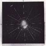
is called a Plan Position Indicator (PPI). Plate 65 shows a photograph of a PPI.
This photograph is a time exposure equal to the
time for one antenna revolution. The center of the photograph is the
location of the radar station. Concentric circles around the center
indicate distance from the station. In this case the range circles
are at 10 mi. intervals, so the total displayed range is 150 mi.
North is at the top of the photograph and lines radiating from the
center are at 10° intervals.
The radar operator must keep watch of this entire area (70,650 sq.
mi. in this example) and try to determine the nature of the targets.
If he is a meteorologist he watches for and tracks weather phenomena
and ignores echoes which are obviously not weather-related. If he is
an air traffic controller he concentrates on those echoes that are
from aircraft for which he is responsible. Many unexplained radar
echoes are not studied or reported for several reasons. One of the
reasons might be that the operators in general only track targets
that they can positively identify and control. Since a radar operator
can only handle a limited number (6 to 8) of targets simultaneously,
he might not take serious note of any strange targets unless they
appear to interfere with the normal traffic he is vectoring. Even
when the unexplained extraordinary targets are displayed, he has
little time available to track and analyze these targets. His time is
fully occupied observing the known targets for which he is
responsible. In addition, the operator is familiar with locally
recurring strange phenomena due to propagation conditions and
suspects the meteorological environment as being the cause. In
general, the operator seldom has a way in which to record the
displayed data for later study and analysis by specialists.
In addition to the tracking of various targets he must also be aware
of the possibility of malfunction of the radar.
Two types of failures occur in a radar system: those that are
catastrophic and those that cause a gradual degradation. In spite of
good maintenance procedures, there will be system component failures
that occur due to external events such as ice or wind loading, rain
It can be considered that a major system component of a typical radar
might be subject to catastropic failure every 250 to 2,000 hours of
operation (5 to 36 average failure-free days) and that graceful
degradations of components occur continually. Possible failure thus
becomes one of the first causes to be considered in analyzing unusual
radar sightings. The next factor will be possible unusual propagation
effects to which the radar is subject. Analysis of extraordinary
sightings is further handicapped by the fact that the displayed data
of the sighting usually are not recorded and that any explanations
must frequently be based upon interpretations by the operators
present at the time of the sighting. The point is that the operator,
the radar, and the propagation medium are all fallible parts of the
system.
There are five possible relationships between radar echoes and
targets. These are:
The situations (c.) where there is an apparent echo but no target are
those when the manifestation on the PPI is due to a signal that is
not a reradiated portion of the transmitted pulse but is due to
another source. These are discussed in a subsequent section of this
chapter.
Situations where the echo is from a target not at the indicated
location (d.) may arise due to one or a combination of the following
reasons. First, abnormal bending of the radar beam may take place due
to atmospheric conditions. Second, a detectable target may be present
beyond the designed range of the radar and be presented on the
display as if it were within the designed range, for example,
multiple-trip echos from artificial satellites with large radar
cross-sections. Third, stray energy from the antenna may be reflected
from an obstacle to a target in a direction quite different from that
in which the antenna is pointed. Since the echo is presented on the
display along the azimuth toward which the antenna is pointed the
displayed position will be incorrect. Finally, targets could be
detected
Possibility (e) listed above encompasses the broad range of
situations where there is a target at the location indicated on the
display system. Of primary concern in this case is the identification
of the target.
The possible relationships listed above show that radarscope
interpretation is not simple. To attempt to identify targets, the
operator must know the characteristics of his radar; whether it is
operating properly; and the type of targets it is capable of
detecting. He must be very aware of the conditions or events by which
echoes will be presented on the radar in a position that is different
from the true target location (or in the case of interference by no
target). Finally, the operator must acquire collateral information
(weather data, transponder, voice communication, visual observations
or handover information from another radar before he can be
absolutely sure he has identified an unusual echo.
Sources of electromagnetic radiation that may cause real or apparent
echoes on the radar display include both radiators and reradiators.
Some sources, such as ionospheric electron backscatter, the sun, and
the planets, are not considered, since they can be detected only by
the most sensitive of research radars. As a radiator the sun does
emit enough energy at microwave wavelengths to produce a noise
signal. This signal has been used for research purposes (Walker 1962)
to check the alignment of the radar antenna. Radio sextants have been
built which track the sun at cm. wavelengths by Collins Radio Co.
Since this signal is quite weak it is unlikely it would be noticed
during routine operation of a search radar.
Reradiators include objects or atmospheric conditions that intercept
and reradiate energy transmitted by the radar. Objects range in size
from the side of a mountain to insects. Atmospheric conditions
include ionized regions such as those caused by lightning discharges
In the 1940's when radar technology advanced to the point where
wavelengths less than half a meter began to be feasible,
precipitation became a radar-detectable target. Ligda (1961) states
that the first radar storm observation was made on 20 February 1941
in England with a 10 cm. (S band) wavelength radar. Since that time,
radar has been widely used for meteorological purposes and special
meteorological radars have been designed and constructed specifically
for precipitation studies (Williams, 1952; Rockney, 1958). Many
radars designed for purposes other than weather detection were found
to be very adequate as precipitation detectors. Ligda (1957) studied
the distribution of precipitation over large areas of the United
States using PPI photographs from Air Defense Command (ADC) Radars
during the period 1954 to 1958 and during 1959 studied the
distribution of maritime precipitation shown by PPI photographs from
radars aboard ships of Radar Picket Squadron I stationed off the west
coast of the United States. Later programs concurrent with several of
the meteorological satellites (Nagle, 1963; Blackmer 1968) have also
utilized data from ADC and Navy radars. Thus radars designed for
other specific missions are often capable of detecting precipitation
and an understanding of the characteristic behavior and appearance of
precipitation is essential if the radar operator is to interpret
properly the targets his radar detects.
Detailed studies have been made of characteristics of radar returns
from precipitation. In a review of the microwave properties of
precipitation particles Gunn and East (1954) discuss variations in
return signal with wavelength and differences between the return
signal from liquid and frozen water particles. Precipitation consists
of a large volume of particles that generally fill the beam at
moderate ranges. The
Radar-detected precipitation may be in a variety of forms from very
widespread continuous areas of stratiform precipitation of sufficient
vertical extent to nearly cover the PPI of a long-range (150 n.mi.)
search radar to only one or two isolated small sharp edged convective
showers. The former is likely to persist for many hours, the latter
for only a fraction of an hour. Between these two extremes there are
many complex mixtures of convective and stratiform precipitation
areas of various sizes. One of the distinguishing features of
precipitation echoes is their vertical extent and maximum altitude.
Usually precipitation echoes extend from the surface to altitudes up
to 60,000 ft., although a more common altitude of tops is 20,000 -
40,000 ft. Further, isolated small volumes of precipitation seldom
remain suspended in the atmosphere. The initial echoes from showers
and thunderstorms may appear as small targets at moderate altitudes
but subsequently grow
Since precipitation is less detectable at longer wavelengths and
showers may have a quite short lifetime, it is possible that on rare
occasions precipitation targets could confuse the radar operator.
Consider for example a search radar operating at wavelengths of
greater than 20 cm. in an environment where short-lived showers were
occurring. A study by Blackmer (1955) using photographs from a 10 cm.
radar showed a peak in echo lifetimes of 25 - 30 min. while the mean
lifetime was 42 min. Also using data from an S band radar, Battan
(1953) found a mean echo duration of 23 min. with the greatest number
having lifetimes of 20.0 - 24.9 min. At longer wavelengths with short
lifetimes, it is not impossible that an intense shower would be
detectable only in the brief period during which it was producing
hail, because a long wavelength radar might not detect small
precipitation particles but could detect hail. Water-coated hail acts
as a large water sphere and thus gives very strong return signals
even at long wavelengths. Geotis (1963) found that hail echoes are
very intense subcells on the order of 100 M. in size. When a number
of short-lived showers or long-lived showers that were detectable
only when hail is falling, are within range of a long wavelength
radar, the PPI display could show over a period of time, a brief echo
at one location, then an echo at a new location for a
One of the characteristics of precipitation echoes is that their
motion is very close to that of the wind direction and speed. This
wind velocity may not be the same as that observed at the radar site
if the distance to the precipitation is great. Occasions have also
been noted when precipitation echoes within a relatively small area
have shown differences in motion due to being moved by different wind
directions at various levels.
In general, however, precipitation is a relatively well behaved radar
target and except for rare instances its extensiveness and orderly
movement readily identifies it to the radar operator monitoring a PPI
display.
The term aircraft includes a wide variety of vehicles from unpowered
sailplanes to the most advanced military jets with speeds several
times that of sound. A target such as an aircraft has a very complex
shape that is many times the wavelength of the incident radar energy.
As the energy scattered from different parts of the aircraft adds or
subtracts from other parts, the signal returned to the radar
fluctuates. Fluctuations in the echo can also result from changes in
the angle at which the aircraft is viewed. That is, when an aircraft
is viewed broadside, its radar (and visual) cross-section is much
larger than when viewed from the nose or tail. Skolnik (1962) reports
a 15 dB change in echo intensity with an aspect change of only 1/3 of
a degree. High frequency fluctuations due to jet turbines (Edrington,
1965) and propellors (Skolnik, 1962) have also been reported. These
fluctuations are on the order of 1000 cycles per second and would not
be apparent on a PPI.
Although aircraft echoes fluctuate due to aspect and propulsion
modulations, there is a general correlation between size of aircraft
and the amount of signal returned to the radar. An indication of the
The radar cross-sections of components of a large jet aircraft was
measured with a 71 cm. radar (Skolnik 1962) and maximum values in
excess of 100 m2 were found. The fuselage of the large jet
when viewed from the front or rear had a cross-section of about
one-half square meter. Smaller aircraft would have much smaller radar
cross-section of about one-half square meter. Smaller aircraft would
have much smaller radar cross-sections and light aircraft or
sailplanes of fiberglass or wooden construction could have extremely
small radar cross-sections.
Another type of fluctuation in echo signal from aircraft and similar
point targets is due to the nature of radio wave propagation. When a
radar wave is propagated over a plane reflecting surface there will
be reflections from that surface to a target in addition to the
direct path from the radar to the target. Figure 3 illustrates the
geometry of beam distortion due to such a plane reflecting surface.
In Fig.3a an idealized beam pattern in free space is shown. When a
reflecting surface such as the ground or sea surface is introduced a
portion of the beam will be reflected from the surface as in Fig.3b.
A target will thus be illuminated both by a direct wave and a
reflected wave. The echo signal from the target back to the radar
travels over the two paths so that the echo is composed of two
components. The resulting echo intensity will depend on the extent to
which the two components are in phase. Areas along which the two
components are in phase resulting in a stronger signal lie along
lines of angular elevation of
The effect of these fade areas is to cause aircraft targets to
sometimes disappear and then (if the target has not reached a range
such that the return signal is no longer detectable) to reappear.
With a number of aircraft flying about it is not inconceivable that
the fadings and reappearances of the several aircraft would be
difficult to keep track of and could be misinterpreted as a smaller
number of targets that were moving quite erratically.
Considering the whole spectrum of vehicles that travel in the
atmosphere, there may be speeds as low as zero (hovering helicopter)
or speeds exceeding Mach 3.0. Correspondingly, altitudes vary from
the surface to 50,000 - 60,000 ft. (in some cases above 100,000 ft.)
Different types of aircraft, however, are limited in their range of
speeds and altitudes. A hovering helicopter cannot suddenly
accelerate to three times the speed of sound. Neither can a
supersonic jet hover at 60,000 ft. A characteristic of an aircraft
echo on a PPI is therefore its relative uniformity of movement. To
monitor this movement allowance must be made for fades. The direction
of movement also will be quite independent of wind direction at
flight level.
Possibly the earliest observation of a radar echo from a bird was
made by R. M. Page (1939) of the Naval Research Laboratory in
February, 1939. It was made with an experimental 200 MHz. radar (the
XAF) on the U.S.S. New York near Puerto Rico. Bird echoes, as
reported by Lack and Varley (1945), were observed on a 10 cm.
coast-watching radar set near Dover during 1941. Visual checks
confirmed both of these early detections by radar as being returns of
individual birds. Numerous bird observations by radar have been made
since,
Because of the inverse-fourth-power variation with range, a bird at
short range in the main beam can give a radar echo comparable in
intensity to that from an aircraft in the main beam at a long range.
For example, if a pigeon with a broadside radar cross-section of
100 cm2 were flying within the radar main beam at a
range of 10 mi., it would produce as strong a signal to the radar as
a jet aircraft with a a value of 106 cm2
(100 m2) flying within the radar main beam at a range
of 100 mi. However, if the aircraft were flying in a side-lobe 40 dB
less powerful than the main beam in which the bird is flying both
would produce equal intensity signals at the same range. If the side
lobe were 30 dB down, a bird in the main beam at 10 mi. would look
like an aircraft at 17.8 mi., and if the side lobe were 20 dB down,
the bird at 10 mi. would look like an aircraft at 31.6 mi.
Theoretically the maximum detectable range as dictated by the amount
of radar signal returned from birds can be calculated. However,
verification is not easy due to the difficulty of spotting a bird and
establishing that it belongs to a particular blip on a radar scope.
This is particularly difficult in the presence of sea clutter as
experienced during an experiment conducted by Allen and Ligda (1966)
at Stanford Research Institute. During an experiment conducted by
Konrad (1968), individual birds were released from an aircraft flying
over water at 5,500 - 6,000 ft. from 8 - 10 n.mi. from the radars.
After separation of the aircraft from the bird in the radar scope,
each individual bird was automatically tracked for periods up to five
minutes, so that the target observed was positively identified as a
bird. Flocks of birds have been detected to ranges of at least 51
n.mi. as reported by Eastwood and Rider (1965).
Grackle Grackle Sparrow Sparrow
†VH, Transmit vertical polarization and receive cross-polarized
or horizontal component.
†400 megacycles.
Eastwood and Rider (1965) reported a rather complete analysis of the
height of flight of various birds observed by radar at the Marconi
Research Laboratory in England. Their findings agreed very closely
with the above; about 90% of all birds were below 5,000 ft. Birds fly
higher at night and during the spring and fall migration periods. A
plot of the average altitude distribution over the year is shown in
Fig. 4. All of these figures are probably applicable as height above
the general terrain; i.e., at 5,000 ft. above mean sea level, 90% of
the birds would fly at altitudes below 10,000 ft.m.s.l. The amount of
cloud cover also affects the height at which birds fly. Diagrams
included by Eastwood and Rider (1965) clearly indicate a marked
tendency for higher mean altitudes to be flown in the presence of
complete cloud cover.
Target airspeed is another means for identifying a bird. It can be
obtained vectorially from a knowledge of the wind velocity and the
radar-measured target velocity. Houghton (1964) determined the
airspeed of a limited sampling of the birds by visually identifying
each through a telescope aimed by tracking radar Fig. 5. In all cases
the wind speeds were less than 5 knots. Target air speed cannot
invariably distinguish between a helicopter, a slow moving aircraft
and a bird flying in a high wind without precise knowledge of the
wind at the bird altitude.
Under some conditions, slow-moving ring echoes may be produced by the
rise of a temperature inversion layer in the early morning hours
after sunrise. Sea-breeze fronts have occasionally been seen on radar
as a line, and at other times as a boundary between scattered and
concentrated signal returns as shown by Eastwood (1967). How much of
the line produced is due to the meteorological effects and how much
by birds and insects is still a matter for speculation. However,
Eastwood (1967) cites reports by glider pilots sharing upcurrents
with birds taking advantages of the lift provided. This and some
limited study of the characteristics of the radar scope signals,
produce some indication as to the validity of the bird theory.
Some studies have been made on target signal fluctuation and other
signature analysis techniques in connection with birds (Eastwood,
1967) and even with insects (Glover, 1966). Some of the signal
characteristics have been attributed to aspect of the target and
others to wing motion. There is ample evidence that insects are to be
found in the atmosphere well above the surface. Apart from flying
insects, creatures such as spiders can become airborne on strands of
gossamer and be borne aloft in convective air currents. Glick (1939)
reports in considerable detail the results of collecting insects from
aircraft over the southern U.S. and Mexico. He found concentrations
of insects of the order 1 per
The radar cross-sections (sigma) of the various insects listed in
Table 4 (measured at wavelenths of 3.2 cm.) range from 0.01
cm2 to 1.22 cm2 for all but the locust which
has a maximum sigma value of 9.6 cm2. The ability of any
given radar system to detect radar cross sections of these low values
is a function of its design, its current performance, and the ability
of the operator. Ultra-sensitive radar systems such as the MIT
Lincoln Laboratory radars at Wallops Island, Va. have reported
minimum detectable cross-sections at 10 km. of 6x10⁻⁴
cm2 for the X-band, 2.5x10⁻⁵ cm2 for
the S-band, and 3.4x10⁻⁵ cm2 for the UHF radars
(Hardy, 1966). The X-band radar is two orders more sensitive than
required to detect the listed insects at a range of 10 km. and
probably is functioning close to the limit of detectability. The
majority of other radar systems in general use today are less
sensitive. Some are not able to detect insects in the lower range of
a values. Tabulation of a large number of radar system
characteristics has been published in classified documents by RAND.
Major radar parameters for some airborne sets are listed in an
article by Senn and Hiser (1963)
Insects are commonly found at surprisingly high altitudes. Swarms of
butterflies and other insects are found in summer on 14,000-ft.
mountain peaks in the Rockies. A few insects have been reported at
over 25,000-ft. altitudes in the Himalayas.
Verification of insects as causing a particular blip on a radar scope
is even more difficult than birds. Flowever, this was accomplished as
reported by Glover, et al (1966). Single insects were released from
an aircraft and tracked by radar at altitudes from 1.6 to 3.0 km. and
at ranges up to 18 km. Experiments of this sort and other studies
involving clear atmosphere probing with high-power radars (Atlas,
1966; Hardy, 1966 and 1968) have led to valid conclusions that most
of the dot echoes are caused by insects or birds.
Attention has been given by Browning (1966) to the determination of
Three kinds of angel population were distinguished according to their
mean deviation from the swarm velocity, their average vertical
motion, their maximum relative velocities and their sigma values.
Atmospheric inhomogeneities or the presence of plant seeds appeared
to be ruled out because of the small back-scattering cross-sections
of individual angels (less than approximately 0.1 cm2),
their discreteness in space and velocity, their often quite large
mean deviations (up to 4 m sec-1) from a uniform velocity,
and the fact that the only major upward velocities occurred after
sunset, at a time when the lapse rate was becoming increasingly
stable. The same data suggest insects as the likeliest cause.
Some of the larger man-made objects in space (such as the Echo I and
Echo II metallized balloons, Pegasus, and large boosters) have large
radar cross-sections and can be detected by search
radars*. For example, Peterson, (1960) found that
occasionally the radar cross-section of Sputnik II approached
1000 m2. Such space objects at altitudes of around
120 mi. and with speeds of around 18,000 mph could appear as multiple
trip echoes if they were detected on a search radar.
Fig. 6 illustrates the possible appearance of the track of a
satellite on the PPI of a search radar. The figure assumes a
satellite at 120 n. mi. altitude moving radially at a distance of 500
n. mi. from a radar with an unambiguous range of 200 mi. (The
elevation angle of the satellite would be about 8° which is
within the vertical coverage of many search radars.) When the
satellite is at point A the echo is displayed on the PPI at point A',
400 mi. less than the actual range. As the satellite moves to point B
its range closes to less than 450 mi. so the echo moves to within 50
mi. on the PPI. From B to C the range of the satellite opens to 500
mi. so the echo moves
NCAS EDITORS' NOTE: This footnote was listed on the errata
sheet, but not the text to which it applies; we have placed the
asterisk on the page at a spot that seems reasonable from the
context.
Detection of satellites by search radars would therefore result in
high-speed echoes on the PPI. If the satellite were moving toward the
radar the echo would move at the satellite velocity but would
probably be detected for a shorter period since as it approached the
radar it would rise above the vertical coverage of the radar beam.
In 1906 J.J. Thomson showed that ionized particles are capable of
scattering electromagnetic waves. Sources of ionized particles
include lightning strokes, meteors, reentry vehicles, corona
discharges from high voltage lines, and static discharges from high-
speed aircraft. Ionospheric 'layers and the aurora are also
ionization phenomena. These ionization phenomena or plasmas may under
certain conditions produce radar echoes on the PPI of a typical
search radar.
Plasmas resulting from lightning discharges return echoes which may
be seen on the PPI if the operator is looking at the right spot at
the right time. A number of investigators (Ligda, 1956; Atlas 1958a)
have discussed the appearance of lightning echoes on the PPI. The
echoes typically vary from a point to irregular elongated shapes up
to 100 mi. or more in length.
The radar cross-section of the ionized column of plasma produced by
lightning has been estimated by Ligda (1956) to be 60 m2
depending on ion density within the plasma and on the wavelength of
the radar illuminating the plasma. Electron densities of
1011/cc are required for critical (100%) reflection of 3
cm. radar energy; only 109 electrons / cc are required
with a 30 cm. radar. Thus, longer wavelength radars are more apt to
detect lightning than the shorter wavelength radars. There is another
factor which aids lightning detection at longer wavelengths. The
longer wavelength radars detect less precipitation than the shorter
wavelength radars. Therefore, a lightning discharge inside an area of
light precipitation might be hidden within the precipitation echo on
the PPI of a 3 cm. radar, while a 23 cm. radar might detect the
lightning-produced plasmas but not the precipitation.
Confirmation that short-lived (one scan) echoes were caused by
lightning was based on the fact that there were visual lightning
discharges in the area from which the radar received the echoes.
Atlas (1958a), however, estimated (from echo intensities and
dimensions) that discharges may occur that are radar detectable, but
are not visible to the eye. Whether or not there is visible lightning
in the area of these short echoes, there will undoubtedly be
precipitation areas in the vicinity. The exact distance from
precipitation that lightning may occur has not been adequately
studied. It is known that the probability of radar detection of
lightning is greatest when the radar beam intercepts the upper levels
(ice crystal regions) of thunderstorms. In a mature thunderstorm the
ice crystal blowoff or anvil may extend many tens of miles downwind
of the precipitation area. Atlas (1958a) illustrates a lightning echo
some 10 to 20 mi. ahead of the precipitation echo but within the
anvil cloud extending downwind from the storm.
Since search radars can detect echoes of very short duration returned
by plasmas created by lightning flashes, there is no reason to assume
that other plasmas could not be detected by search radars if the
plasmas were sufficiently separated from other targets. The radar
echoes would probably appear as point targets and if the duration
were sufficient to compute a speed, it would correspond to that of
the plasma. The possible range of speeds of plasma blobs cannot be
given since so little is known about the phenomenon.
In addition to reflections of the radar pulse there is another source
of signals from the lightning discharge, those that are radiated by
the lightning discharge itself. These signals, called sferics, appear
on the PPI as radial rows of dots, as one or more short radial lines,
or as a combination of dots and lines (Ligda,1956). Atlas (1958b)
states that 10 cm. and 23 cm. radars are good sferics detectors while
radars such as the 3 cm. CPS-9 have moderately low range capabilities
in detecting sferics.
As with the lightning echo, the sferic duration is very short Atlas
(1958b) found an average 480 microseconds for 489 sferics measured
during a severe squall line on 19 June 1957. As a result such sferic
signals from a given lightning discharge would only be displayed on
one scan of the PPIL.
The aurora is a complex phenomenon caused by ionization of the upper
atmospheric gases by high-speed charged particles emitted by the sun.
Upon entering the earth's upper atmosphere, these charged particles
are guided by the earth's magnetic field and give rise to
Increased auroral activity is found to follow solar magnetic storms.
A direct correlation exists between sunspot activity and the
intensity and extent of aurora. The increased auroral activity
follows a solar disturbance by about one or two days, the time
required for the charged particles to travel from the sun to the
earth. During these times, auroras may be seen at latitudes far
removed from the normal auroral zones.
Auroral displays occur in the ionosphere at altitudes ranging from
54-67 mi. The ionization which is seen as a visual auroral display is
formed into long slender columns which are aligned with the earth's
magnetic field. This formation results in strong aspect sensitivity
which means that radar reflections occur only when the radar beam is
approximately at right angles to the earth's magnetic field. Echo
strength is proportional to the radar wavelength raised to the third
or fifth power; consequently, most radar observations occur at VHF or
lower UHF.
As a result only lower frequency UHF search radars within 1000 mi. of
the Arctic or Antarctic Circles would be capable of detecting auroral
echoes. The echoes would generally appear at true ranges of 60 - 180
mi. for a few minutes to several hours. The echoes would be mainly
stationary and could be either distributed or point targets usually
in the magnetic north azimuths in the northern hemisphere or magnetic
south azimuths in the southern hemisphere.
Meteors are small solid particles that, when they enter the earth's
atmosphere, leave an ionized trail from which radar echoes are
returned. The majority are completely ablated at altitudes ranging
from 50 - 75 mi. Visible meteors vary in size from about 1 gm. to
about 1 microgram. The ionized trail produced by a 0.1 gm. meteor is
miles long and only a few feet in diameter.
Although most meteor echoes last no more than a fraction of a second
when observed with VHF radar, a few echoes persist for many seconds.
The duration of the meteor echo is theoretically proportional to the
square of radar wavelength, and the power returned is proportional to
the wavelength cubed. For these reasons, meteor echoes are seldom
detected at frequencies above VHF.
Meteor echoes on a low frequency UHF radar usually appear as point
targets with a duration of a few seconds or less. Ranges center
around 120 mi.
Very, very infrequently meteors occur that are large enough to
survive atmospheric entry. They usually produce a spectacular visual
display, referred to as fireballs. Such meteorites are detectable by
sensitive search radars operating at any frequency and at any angle
to its path. Echoes appear as point targets with a duration of a few
seconds. The true range would be less than 120 mi. and the range rate
generally would be less than 20,000 mph.
Balloons and instrument packages or reflectors carried by balloons
can be detected by search radars. More than 100 balloons are released
over the United States at least twice a day from Weather Bureau,
Navy, and Air Force Stations for the measurement of upper atmospheric
conditions. A number of these balloons carry radar reflectors as well
as an instrument package, and some are lighted for theodolite
(visual) tracking. Echoes from these point targets move at the speed
of the wind at the altitude of the balloon. Balloon altitudes vary
widely and may reach 100,000 ft. so that ground speeds vary from near
zero to well over 100 knots. When a balloon bursts and the instrument
package abruptly starts a descent which is normally slowed by
When radar was developed as a means for aiming searchlights and
antiaircraft guns during World War II, countermeasures were promptly
devised. What was needed was something inexpensive and expendable
that would give a radar return comparable with the echo from the
aircraft. Small metallic foil strips which act as dipole reflectors
were employed. The strips are released from an aircraft, and they are
wind-scattered which results in a cloud with a radar cross-section
comparable to a large aircraft.
The terms "chaff," "window," and "rope" are used to designate
particular types of materials. Chaff consists of various lengths of
material. Chaff having the same length is called window. Rope is a
long roll of metallic foil or wire designed for broad, low frequency
response.
Metallized nylon monofilaments have replaced metal foil in the
construction of chaff and window. The nylon type is lighter, hence
has a slower rate of descent, and is more compact. A typical package
of X-band chaff is a cylinder 1 in. in diameter and 1.5 cm. (one half
the 3 cm. wavelength) long. The cylinder contains approximately
150,000 filaments and weighs 6.5 gm. and forms a cloud with a radar
cross-section of about 25 m2. The filaments descend at
about 2 ft/sec in still air at lower altitudes, so that if dispensed
at 40,000 ft. they take about four hours to reach the ground.
Turbulence causes the chaff cloud to grow and disperse, so that
generally the signal becomes so much weaker that sometimes the chaff
cloud cannot be tracked all the way to the ground.
Rope is a 60 - 80 ft. piece of narrow metallized material such as
mylar. It is weighted at one end and has a drag mechanism at the
other. When deployed it has a rate of descent about twice as fast as
chaff so it would take about two hours to fall from 40,000 ft. to the
surface. Usually a number of rope elements are deployed together so
there will be some increase in the size of the cloud as it descends.
Hiser (1955) reports detecting smoke from fires at a city disposal
dump about 15 mi. from the site of a 10 cm. search radar. The radar
echo from the smoke plume was evident on the PPI extending in a
northeasterly direction to a range of 50 mi. Goldstein (1951)
mentions a case where an airplane was directed to an echo observed by
a 10 cm. radar. Only several columns of smoke from brush fires were
found. Smoke particle size and concentrations are so small that one
would be highly skeptical about echoes from the smoke itself. The
returns may arise from refractive index discontinuities at the
boundaries of the smoke plume. Plank (1956) suggests that echoes from
the vicinity of fires may be from either particles (neutral or
ionized) carried aloft by convective currents or from atmospheric
inhomogeneities created by the fire.
Local terrain features and, at sea, the ocean surface are detected by
radar. The range to which such clutter is detected is a function of
antenna height, elevation angle and beamwidth, and the distribution
of temperature and humidity along the propagation path.
To investigate the phenomena of distant ground return it is first
necessary to review some of the fundamentals of the propagation of
electromagnetic radiation through the atmosphere. The interested
reader can find a comprehensive treatment of tropospheric radar
propagation in a book on radio meteorology by Bean (1966) which
covers in detail the topics in the following brief review.
In a vacuum, electromagnetic energy is propagated in straight lines
at the velocity of light, 3x10⁸ m/sec. This constant is
usually designated by the symbol "c." In a homogeneous medium, the
direction of propagation remains constant, but velocity (V) is
reduced and
(1)
The angle of the incident ray (theta) is related to the angle of the
refracted ray (theta') by the equation:
(2)
The ray is always refracted towards the medium of higher refractive
index. A portion of the energy will also be reflected in the same
plane and at an angle equal to the angle of incidence if the energy
encounters a sudden change in the refractive index; this is a partial
reflection. Total reflection occurs when the angle of incidence
exceeds a critical value given by (with n1 < n):
(3)
(3)
where nh is the refractive index at height h,
ns is the refractive index at the surface, a is the radius
of the spherical earth, beta is the ray elevation angle at height h
and beta0 is the ray elevation angle at the earth's
surface (See Fig. 7).
A most important consequence of this is that the effects of a
vertical gradient of refractive index are most apparent at low
(10° or less) angles of elevation.
Where the refractive index gradient is constant
In terms of the real atmosphere, at radar frequencies the refractive
index varies as a function of pressure, temperature, and water vapor
content. An equation relating the various parameters as given by
Smith (1953) is:
For convenience, the left-hand side of the equation is commonly
designated N (refractivity) and is expressed in equation is commonly
N-units, i.e., N = (n - 1) 106.
At sea level, a typical value of n is 1.00035, i.e., the refractivity
is 350 N units. But depending upon pressure, temperature and humidity
the sea level refractivity may range from 250 to 450 N units.
Since pressure, temperature, and water vapor normally decrease with
height the refractivity normally decreases with altitude. In a
'standard' atmosphere, typical of temperate latitudes (with a thermal
lapse of 2°C/1000 ft. and uniform R.H. of 63%, the gradient
(lapse rate) of refractivity is 12 N-units/l000 ft. 39 N.
km-1 in the lower levels. For a constant gradient of this
magnitude, a ray will have a curvature of about 1/4th that
of the earth's surface (the radar horizon in this case is about 15%
further than the geometrical horizon). For short distances the
geometry is equivalent to straight-line propagation over an effective
earth with a radius 4/3 as large as the true earth.
A device frequently used to facilitate the consideration of
propagation geometry and radar coverage takes advantage of this fact.
If a fictitious earth radius is adopted that is 4/3 the earth's true
radius, radar rays in the standard atmosphere may be drawn as
straight lines, which will preserve the same relationship to the
redrawn earth's surface as is the case in reality.
In atmospheres having different constant gradients of refractivity
appropriate factors may be applied to the earth's true radius to
accomplish a similar result. Typical values ire given in Table 5.
(7)
Procedures based on these relationships may be used to trace the path
of rays to determine the detailed effect of refraction on radar
propagation under any given condition of atmospheric stratification.
The broad pattern of refractive effects, however, is as follows:
This condition gives rise to marked anomalies in propagation and,
provided the layer through which such a gradient occurs is deep
enough, the radar energy will be guided within a duct bounded by the
earth's surface and the upper level of the layer. In such cases,
exceptionally long detection ranges are achieved, well beyond the
normal radar horizon (See Fig. 8). Where a marked negative refractive
gradient occurs in a layer adjacent to the ground, a surface duct is
formed (Fig. 9a). An elevated layer of strong negative gradient can
also produce ducting (Fig. 9b).
Surface ducts are commonly caused by radiative cooling of the earth's
surface at night, leading to a thermal inversion in the air near the
surface. In this case, the extreme refractivity gradient is mainly
due to temperature effects and such ducts can occur in quite dry air.
Where humidity at the surface is higher than usual and falls off
rapidly with height, a strong negative refractivity gradient is also
established. Evaporation from water surfaces or wet soil can produce
these conditions and a particularly common example occurs in warm dry
air from the land when it is advected over the sea. This type of duct
is commonly found in tropical areas, where temperature and humidity
both decrease with height; the inversion type of duct is more common
in temperate and artic areas (Bean, 1966).
Elevated layers of extreme refractivity gradient are caused by
similar meteorological mechanisms but often occur on a somewhat
broader scale. Certain areas of the world are particularly prone to
such layers; the California coastal area is a good example.
Plate 66 (Blackmer, 1960) shows an example of the PPI during a trapping
situation off the California coast.
Anomalous propagation of the type described is also significant in
determining the distribution of energy within the envelope of the
main beam, particularly in broad vertical beam systems. At low angles
some energy within the beam impinges on the earth's surface near the
radar and is reflected, still within the envelope of the beam.
Because the path followed by such energy is necessarily longer than
the direct path and because of the wave nature of the energy,
in-phase and out-of-phase interference will occur, leading to a
vertical lobe structure in the beam envelope (see Fig. 10). Anomalous
propagation conditions can readily produce variations in the normal
distribution of energy within the beam due to this mechanism and thus
can easily lead to unexpected variations in signal intensity from
distant targets.
It is important to recognize the difficulties that are inherent in
establishing whether propagation conditions are anomalous in certain
cases. Where the gradient of refractivity extends uniformly over
large horizontal areas, there is little difficulty in determining the
situation either from conventional meteorological data or from the
manifestation of the anomalous performance of the radar itself (for
example, the detection of ground clutter to abnormally large ranges).
In some cases it is possible to infer, with some confidence, from the
meteorological conditions (especially if data on the vertical profile
of temperature and humidity are available) that anomalous propagation
is not present. In many cases, however, the causative
conditions may be very variable in space and time, and it is then
difficult to be at all confident
It is often possible to infer only the likelihood or improbability of
anomalous propagation conditions by reference to the general
meteorological conditions that prevail. Thus one would expect normal
propagation in the daytime in a well-mixed, unstable airstream with
moderate winds over a dry surface, while expecting marked
superrefraction over moist ground during a calm clear night following
the passage of a front that brought precipitation in the late
afternoon.
Localized conditions favorable for superrefraction are also caused by
showers and thunderstorms (Ligda, 1956). The cold downdraft beneath
thunderstorms can cause colder air near the surface than aloft while
evaporation from the rain and rain-soaked surface, causes locally
higher humidities.
In addition to the detection of distant ground targets by refraction
of the radar beam, there is the possibility of reflection or forward
scatter of the beam to ground targets. Whether or not layers that
would reflect the beam to-the ground would also be detected by the
radar has been part of the controversy concerning the nature of
invisible targets in clear air. These so-called "angel" echoes have
been observed since the early days of radar (Plank, 1956; Atlas, 1959
and 1964; Atlas, 1966a). Detailed case studies of selected angel
situations illustrate the difficulty of determining the nature of the
targets causing the angel echoes. For example, Ligda and Bigler,
(1958) discuss a line of angel echoes coincident with the location of
a cloudless cold front. They discuss the likelihood that the line was
due to differences in refractivity
Atlas (1959) studied in detail a situation at Salina, Kans. on 10
September 1956 where cellular and striated echoes covered much of the
PPI to ranges of 85 mi. He concluded that the echoes were due to
forward scatter from a patterned array of refractive index
inhomogeneities to ground targets and back. Recently Hardy and Katz
(1968) discussed a very similar radar pattern. They concluded that
insects were responsible for the echoes and that cellular pattern of
insects was due to atmospheric circulation. Atlas (1968c) agreed that
insects may be responsible for some echoes but that the forward
scatter explanation is valid in other instances.
Investigations of angel echoes with high-power, high-resolution
radars at three different wavelengths have made it possible to learn
much about the nature of targets producing various types of angel
echoes. Simultaneous observations at 3 cm., 10.7 cm., and 71.5 cm.
with the ultrasensitive MIT Lincoln Laboratory Radars at Wallops
Island, Va. have been described by Hardy, Atlas, and Glover (1966) ,
Atlas and Hardy (1966a), and Hardy and Katz (1968a). They found two
basic types of angel echoes: dot or point echoes and diffuse echoes
with horizontal extent. The dot angels are incoherent at long ranges
or when viewed with broad beams but are discrete coherent echoes when
viewed by a radar with high resolution. They may occur in well
defined layers and may have movements different from the wind at
their altitude. Their cross-sections and wavelength dependence are
consistent with radar returns to be expected from insects. Since no
other explanation fits all the observations of these dot angels, it
is concluded that the targets are insects.
(10)
Radars of the type normally used for tracking and surveillance are
unlikely to detect such layers. On the other hand, it has been
suggested that on occasion at low levels where marked intermixing of
dry and moist air is present, dielectric inhomogeneities will be
sufficiently marked and be present in sufficient quantity to produce
detectable echoes with radars of relatively modest performance.
It is conceivable that there could be rare occasions when only
isolated atmospheric inhomogeneities existed or when the
inhomogeneities were such that only the most reflective ground
targets were detectable. In such situations only one or two unusual
ground targets would appear on the PPI. Levine (1960), in a
discussion of mapping with radar, points out how certain combinations
of ground and man-made structures act as 'corner reflectors' and
return a much stronger signal to the radar than is returned by
surrounding features. The sides of buildings and adjacent level
terrain, or even fences and level terrain, constitute such
reflectors. He states that in areas where fences and buildings are
predominantly oriented north-south and east-west, the 'glint' echoes
from the corner reflector effect appear at the cardinal points of the
compass and have therefore been called a "cardinal point effect." In
addition, different types of vegetation have different reflectivities
and these vary further according to whether they are wet or dry.
From the above discussion it is obvious that the identification of
targets as being ground return due to forward scatter or reflection
During the past 15 years, electromagnetic compatibility (EMC) has
emerged as a new branch of engineering concerned with the increasing
problems of radio frequency interference (RFI) and the overcrowding
of the radio frequency spectrum. The EMC problem is increasing so
rapidly that considerable engineering efforts are included in the
design, development, RFI testing and production of all new electronic
equipment from the electric razor and TV set to the most
sophisticated of electronic equipments, such as computer and radar
systems. This is true for entertainment, civil, industrial,
commercial, and military equipment. The problems are compounded not
only because the frequency spectrum is overcrowded, but much earlier
generation equipment, which is more susceptible to and is a more
likely source of interference, is not made obsolete or scrapped. New
generation equipment is potentially capable of interaction problems
among themselves, as well as playing havoc with older equipment. Each
year sees new users bringing new equipment into the frequency
spectrum: such as UHF television, garage door openers, automatic
landing control systems, city traffic management and control systems,
and a vast array of new electronic devices being introduced into
tactical and strategic defense systems.
RFI contributes to the information displayed on radar scopes. It is
caused by the radiation of spurious and/or undesired radio frequency
Much interference may be sporadic, producing only a short lived
'echo.' There may be instances, however, when the interference occurs
at regular intervals that could nearly coincide with the antenna
rotation rate so that the spurious echo' might appear to be in
approximately the same position or close enough to it that the
operator would assume there was a target moving across the scope.
Radio frequency interference can enter the radar system in many places:
The photographs in Plate 66 are time exposures of the PPI. The camera
shutter is left open for a full rotation of the antenna so the
photograph is generated by the intensity of the cathode ray tube
electron beam as it rotates with the antenna. This is in contrast to
an instantaneous photograph that would be brightest where the trace
was located at the instant of exposure and, depending on the
persistence of the cathode ray tube, much less bright in other
regions. While the interference in these photographs appears as lines
it would appear as points at any given instant. The lines are
generated by the time exposure as the points move in or outward along
the electron beam. The photographs also show precipitation echoes.
Examination of the photographs shows that the interference does not
mask the larger precipitation echoes to any appreciable extent but
might mask small point targets.
A radar receiver has a limited bandwidth over which it will accept
and detect electromagnetic signals. In this acceptance band, the
receiver reproduces the signals at the receiver output and displays
them on the radar presentation display. Thus any interfering signals
that fall within this band will be detected and displayed by the very
sensitive receiver. In an S-band (2ghz) pulse radar, the typical
bandwidth of the receiver will be 20 - 50 ghz. Any weak signals in
this frequency band will be detected. Even out-of-band signals can
interfere if they are of sufficient signal intensity to overpower the
receiver out-of-band rejection characteristics. For instance, a very
strong out-of-band signal of 10 watts might be typically attenuated
by the receiver preselection filter by 60 db, reducing it to a signal
of -20 db. To the radar receiver,
Increasingly more powerful transmitters and more sensitive receiver
radar systems need even greater relative suppression of unwanted
emission, to prevent the absolute level of out-of-band interference
from rising to intolerable levels, thus causing interference to and
from other electronic systems.
Even if normally operating radars are not affected by this
interference most of the time, the degradation of the radar
components or of nearby systems can cause the temporary increase in
interference at the radar site. Radar personnel are continually
concerned with this problem. Such acts as opening an electronic
cabinet can cause the local RFI to increase sufficiently to create an
RFI nuisance to the radar system.
Each radar system has been designed to fulfill a single class of
target tracking function, being optimized to provide proper and
reliable target data a high percentage of the time. However, all
systems, including radar systems, have their limitations. Thus, it
must be recognized that there will be times when other systems will
interfere, component parts will either gradually degrade or
catastrophically fail, propagation and meteorological conditions will
deviate far from the normal environment, and maintenance and
operating personnel will
Because of radar engineering design limitations, it is not possible
to direct all of the transmitter energy into the main antenna beam
and small but measurable amounts of energy are transmitted in many
other directions. Similarly, energy can be received from such
directions, in what are known as the side lobes of the antenna, and
can give rise to erroneous directional information. Particularly
complicated situations arise when side lobe problems are associated
with building or ground reflection mechanisms. For example, if a
radar antenna is radiating 100,000 watts peak power in the main beam,
100 watts can be simultaneously radiated from a -30 db side lobe in
another direction. Fig. 11 (adapted from Skolnik, 1962) shows a
radiation pattern for a particular parabolic reflector. Note that if
the main beam is radiating 100 Kw, the first side lobe, the first
minor and the spillover lobe radiate about 100 watts. This 100-watt
radiation will be reflected from large targets in this side lobe
heading but will be shown on the PPI as having the same bearing as
the main beam of the antenna. This display of a false target is
called a ghost. In this particular instance two targets having
identical radar cross-sections would appear as returns of equal
intensity if one were in the main beam and the other in the side lobe
but 5.6 times closer to the radar.
Highly reflective targets can often be detected in the side lobes.
Thus a single large target detected in the numerous side lobes can be
displayed in a number of places simultaneously. Since, in radar
displays, target echoes are represented as being in the direction in
which the antenna is pointing, not in the direction from which the
energy is returning at the time of the detection, side lobe echoes
from
Detection from vertical side lobes can cause strange effects when
"radio dusting" is present. Many radars are constructed so that the
antenna cannot be pointed at very low elevation angles, in order to
avoid the most severe anomalous propagation effects or, more often,
to avoid ground reflections. Assume, for example, a radar with a beam
width of (nominally) 1°, having a minimum at say 1.5° and a
side lobe at 2°. Assume also that the antenna is constrained to
elevation angles of 1.5° or greater. If a surface duct is
present, the strongest signals would be attained by pointing the
antenna (and the main beam) at an elevation angle of 0°, but this
cannot be done. However, ducted targets could be detected with the
first (vertical) side lobe, and in this case the maximum AP signals
(ducted) would be attained at an apparent elevation angle of 2°
(so that the main side lobe was at 0°), and the intensity of
these false target signals would decrease or even disappear if the
antenna were lowered to its minimum setting of 1.5°. This sort of
behavior has apparently led some investigators of specific UFO
incidents to discount the possibility of anomalous propagation as the
source of unknown radar targets.
Smith (1962) discusses the effects of side lobes on observed echo
patterns during thunderstorms and periods of anomalous propagation.
In
One effect of such lobes is that when the antenna of a search radar
is elevated (so that at longer ranges no ground return should be
evident) ducted side lobe radiation results in echoes on the PPI.
Without understanding what is happening, the operator would logically
assume a strong target at high altitudes.
Angle of arrival measurements by a radar, like other measurement
devices, will be limited in accuracy by noise and interference. Other
limiting factors can be the reflection caused by the wave
characteristics of electromagnetic radiation. Reflections from the
ground in front of the antenna system or from a nearby building or
mountain can be minimized by proper antenna location. These effects
can seldom be reduced to zero and are detrimental to an extent that
depends on the antenna lobe pattern, geographical, and extraordinary
meteorological conditions, thus causing residual reflection problems.
Another phenomenon explaining strange and erratic radar returns has
been observed with echoes occurring at locations where no targets are
to be found. Analysis of these observations shows that the echoes are
from ground or airborne objects which are being detected by radiation
reflected from mirror-like plane surfaces of vehicles or buildings in
the neighborhood of the radar. If the reflector is moving, then the
reflected ground target behaves like a moving target.
Mechanisms of multiple reflections which serve to produce ghosts are
illustrated in Fig. 12. These involve specular reflection from the
first target, effectively deflecting a significant amount of radar
energy to a second target at a different azimuth, which is oriented
so as to reflect most of the radiation incident on it. Either of the
reflecting targets can be stationary or moving objects. In Fig.12 the
radar is at the point labeled "1." A reflector is a point "2" and
real targets are at the points labeled "3." Due to reflections from
the reflector to the targets, ghost echoes will appear at the points
labeled "4." The appearance of the ghost on the PPI is one possible
explanation for perplexing unidentified target motions. If one of the
two reflectors is an aircraft and undertakes any maneuvers, the path
followed by the ghost is especially erratic. As viewed on a PPI scope
perhaps it first recedes from, then "flies" parallel to, and finally
overtakes or appears to collide or pass the real aircraft.
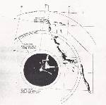
Fig. 13 (adapted from Levine 1960) shows the outline of a
conventional aircraft surveillance radar PPI (included within the
circle). The solid line (A) shows the return echo path of an aircraft
traveling at 300 knots. The dashed line (B) shows the echo path that
will also result when sufficient radar energy is scattered from the
aircraft to a prominent ground reflector located at C, and then
reflected back to the aircraft and then to the receiver. In this
example, the aircraft is the first of the reflectors, so that the
phantom echo always occurs
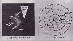
Fig. 13 and the discussion above relate to the case when the aircraft
is the first of two reflectors. For the conditions with the ground
object as the first of the two reflectors, the phantom echo always
occurs at the same azimuth bearing as the ground object. For example,
in Fig. 14 (also adapted from Levine, 1960) the solid line (A)
applies to scattering from the first reflector to the aircraft and
back to the receiver. The inward and outward excursions of this path
actually occur along a single radial line from the radar site through
the first reflector.
In any actual situation, only fractional portions of the ghost echo
paths might be of sufficient signal strength to appear on the
display. Those particular returns that are closest to the ground
object or where the reflector has the most favorable reflecting
properties will most likely be displayed. In a radar detecting only
moving targets, a stationary ground object might not appear as a
target on the scope. Thus, in this manner, the operator's ability to
correlate ghosts to a reflecting surface is considerably reduced,
especially when many known targets are on the display. From Figs. 13
and 14, it is shown that the phantom echo fell outside the display
and then returned during a later portion of the flight. Thus, if only
portions of the phantom track are a detectable signal, and if (this
would usually be the case) there are several targets on the display
at once, the operator would find
In general doubly reflecting ground targets must be of sufficient
size and have good radar-reflecting properties to serve as radar
reflectors. Reflectors can be moving or stationary. Reflectors that
fit this description include sloping terrain, sloping metal roofs,
metal buildings, nearby ground structures, or large trucks and
trailers.
Fig. 13 illustrates the possible sporadic nature of reflection
echoes.
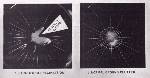
Plate 68a, taken when stratiform precipitation was occurring,
documents the fact that there is a sector to the east that is blocked
by some object. Plate 68b shows normal ground clutter plus a few probable aircraft.
When there is an echo on the PPI of a search radar, the operator must
determine the nature of the target. The information he has is
relative signal intensity, some knowledge of fluctuation in
intensity, position, velocity, and behavior relative to other
targets. In addition he may be able to infer altitude if he is able
to elevate the beam and reduce the gain to find an angle of maximum
signal intensity. Previous sections of this chapter have briefly
described a number of targets that search radars are capable of
detecting. From the discussion it is apparent that there is overlap
in the characteristics of different types of targets. Signal
intensities, for example, range over several orders of magnitude.
Wind-borne and powered targets may have comparable ground speeds
depending on the wind speed. Many different types of targets show
echo fluctuations. Thus there is no specific set of characteristics
that will permit a given echo to be unambiguously identified as a
specific target. At best all one can do is say that a given echo
probably is, or is not, a specific target based on some of the
observed characteristics.
Determination of the direction and speed of an echo in the PPI of a
search radar requires some assumptions. A long range search radar
antenna generally rotates at about 4 - 8 rpm. At 6 rpm, an antenna
rotates through 360° in 10 sec. (=36°/sec). If the horizontal
beam width of the antenna is 3.6° a point target will be within
the beam
The speed computed from the displacement of the echoes from a target
at the indicated location represents the ground speed of the target.
To aid in the identification of slow moving targets. it is necessary
to determine its airspeed. This requires knowledge of the wind
velocity at the location including altitude and time of the
detection, and the assumption that the target is in essentially level
flight. It is often difficult to determine precisely the wind
velocity at a given point due to the wide spacing of stations that
measure winds aloft and the six-hour interval between observations.
Except in complex situations, it is usually possible, however, to
extrapolate measured winds for a given location with sufficient
accuracy to determine whether the target velocity and wind velocity
have sufficient similarity to justify a conclusion that the target is
probably windborne. Conversely if there is a large disparity between
wind velocity and target velocity a logical conclusion would be that
the target could not be windborne.
When an echo that has been moving in an orderly manner on the PPI
suddenly disappears, the information for computing its speed also
disappears. Any attempts to guess the speed would require the
operator to make specific assumptions of the reason for the
disappearance. He might assume that the target moved out of range
during the brief time
The power received from a point target is directly proportional to
the radar scattering cross-section of the target and inversely
proportional to the fourth power of the distance from the radar to
the target. Therefore, for an equal signal to be received from two
targets, a target 10 mi. from the radar would have to have a radar
cross-section 10,000 times as large as a target at 1 mi. Examples of
targets with differences in cross-sections of this order of magnitude
are birds with cross-sections of 0.01 m2 or less and
aircraft with cross-sections of up to 100 m2. Intensity
differences such as these can be measured (by gain reduction to
threshold of detection), but the nature of display systems such as
PPI's is such that differences are considerably reduced. An echo on
the PPI is composed of many small dots that result from an electron
beam that excites the coating on the face of the tube causing it to
emit light. The coating may be designed to emit light only when the
electron beam excites it or may continue to emit light for some time
after the excitation has ceased (persistence). The latter is usually
the case for PPI's where the operator depends on persistence to see
the 360° coverage provided by the rotating antenna. Haworth
(1948) states that from 150 - 200 spots can be resolved along the
radius of magnetically deflected radar tubes. Gunn (1963) points out
that since the PPI trace lines converge at the center the light
output per unit area of the tube face will decrease with increasing
radial distance from the center. As a result echoes near the center
are 'painted' with a higher intensity than echoes of comparable
strength anywhere else on the display. These characteristics of the
display system act to conceal further the relative magnitudes
Very little can be said about a target from the examination of a
single echo but some information can be obtained by comparing the
echo with other echoes on the remainder of the PPI. When the echo is
interpreted in terms of the appearance and behavior of other echoes a
logical explanation may become evident.
For example, the author has seen isolated targets on the PPI that
were moving toward the radar in a direction opposite to that of the
wind, so that it was obvious that they could not be windborne. A
slight elevation of the antenna caused them to disappear so it was
apparent that they were at low levels. No attempt was made to send
aircraft to the vicinity to look for targets. All other attempts to
interpret the nature of real targets on that half of the PPI that
would return the displayed echoes were futile. When the remainder of
the PPI was examined it was found that the speed of a line of
thunderstorms moving toward the station was the same as that of the
echoes to the east. The direction of movement, however, was the same
as that of the wind and not opposite, as with the echoes to the east.
Further, the distance to the thunderstorms to the west was the same
as the distance to the unknown echoes to the east. With this
additional information it seemed likely that the echoes to the east
were reflections
Since the reflectors (chimneys) were very narrow, the reflection
echoes were very narrow but their length was equal to the diameter of
the precipitation area. The echoes therefore had a long, narrow
(cigar-shaped) appearance. Since the apparent lengths in some cases
were 10 - 15 mi. they were not mistaken for some type of flying
vehicle.
Although the solution of the case discussed here is a simple, and, on
the surface, obvious one, it does demonstrate the necessity of
studying the entire PPI, not just one or two odd echoes. The case
also illustrates how echo characteristics become distorted when the
return is from a target not at the indicated location. The long,
narrow shapes of the reflection echoes, a vertical extent of only
1° - 2° at ranges less than 50 mi. and movement against the
wind all tended to rule out precipitation as the target.
The problem of identifying reflections is very difficult. The
simplest case is where the reflector and reflected target are both
fixed. The reflected echo is always in the same position and whether
it appears or not depends on propagation conditions and if the
reflector is of limited vertical extent on antenna elevation angle.
When the reflector is fixed and the target is moving the reflected
echo also moves but in a different direction than the true target.
Still the geometry is relatively simple and the reflected echo will
move toward or away from the radar along a radial line extending from
the radar across the reflector. The reflected echo will appear to
move toward the radar when the distance from the radar to the true
target is decreasing and away from the radar when the distance from
the radar to the true target is increasing. The apparent speed of the
reflected echo toward or away from the radar corresponds to the speed
When the reflector is moving and the target is stationary (see
discussion of Fig. 13) the reflected echo track is always further
from the radar than the reflector track. The reflection echo will
follow roughly the same track as the reflector but its apparent speed
may be much greater depending on the distance between the reflector
and target. When the reflector is far from the target the apparent
speed of the reflected echo will be much greater than the true speed
of the reflector. When the reflector is very close to the target the
reflected echo will be close to the position of the reflector and its
apparent speed will be comparable to that of the reflector.
The situation where both the reflector and the target are moving is
very complex. The apparent speed of the reflected echo will depend on
the relative speeds of both reflector and target. When the reflector
is moving slowly, the condition of a stationary reflector will be
approached but not quite realized. That is, the reflected echo will
have a maximum apparent speed that does not greatly exceed that of
the target, but since the reflector is moving, the reflection echo
will not be restricted to motion along a single radial line.
When the reflector is moving rapidly compared to the target, the
result is similar to the case of a fixed target, that is the
reflected echo track approximates the reflector track but its
apparent speed will be greater. When the target moves, the track
correspondence is not as good and the reflected echo's apparent speed
may greatly exceed that of the reflector.
It is obvious from the preceding discussion that it is nearly
impossible to identify an unknown target working in real time at the
PPI. To establish that an unknown is a reflection echo requires a
determination of whether it is at the same azimuth as a reflector.
Since any one of many other echoes could be the possible reflector,
the geometry would have to be applied to each one in turn. When
numerous echoes are on the PPI this is impossible.
Much valuable information can be recorded for later detailed study by
photographing the PPI with a radarscope camera during each revolution
of the radar antenna. Later the films can be studied, either as
time-lapse motion pictures or frame by frame. For many years this
type of radarscope photography has been used for studies of
radar-detected precipitation patterns and has provided insights into
meteorological phenomena that would have been impossible from
subjective verbal descriptions of the echo patterns.
Radarscope photographs of the PPI have all the limitations of the PPI
presentation itself. They cannot show intensity differences or minor
intensity fluctuations. They do have the powerful advantage of making
it possible to review a puzzling echo hundreds of times at various
rates of viewing and to study the appearance and behavior of all
echoes before, during and after the episode. Only by the study of
radarscope films and many other supporting data is it possible to
arrive at even a tentative conclusion that a given echo cannot be
explained.
Radar is a valuable instrument for detecting and ranging targets that
are not visible to an observer due to darkness, extreme distance,
intervening rain, cloud cover, haze, or smog. Radar can also detect,
or reflect from, atmospheric discontinuities that are not visible to
the eye. The echoes of real targets and apparent targets that result
from RPI, reflections, or system noise may on occasion produce scope
presentations that are extremely difficult or impossible to
interpret. The major difficulty is that while radar is designed to
beam radiation in a specific direction and detect targets within a
specific distance, it does not always do so. The transmitted
radiation, while concentrated in a main beam, goes out as well, in
many other directions. Portions of the main beam and the lobes may be
reflected in other directions by nearby objects, by solid targets a
considerable distance from the radar, or by layers or small volumes
of atmospheric inhomogeneities. All of this radiation in various
directions is refracted by atmospheric temperature and moisture
profiles to deviate further from its original path. Portions of this
radiation that impinge upon any of a wide variety of targets are
reflected back along a reciprocal path and presented on the PPI as if
they were at the position determined by the antenna elevation and
azimuth, and the time required for the most recently transmitted
pulse to travel out and back. Some of the displayed echoes will
represent targets at the indicated locations. Some of the displayed
echoes will be from targets not at the indicated position, and some
of the echoes will not represent targets at all, but will be due to
system noise or RFI. Since radar does not differentiate between the
unique characteristics of different types of targets, it is
impossible for even the most experienced radar operator to look at
the PPI and positively identify all echoes on the scope.
Some auxiliary information on the possible nature of the targets may
be derived from the study of the appearance of the PPI on successive
antenna revolutions or from a series of PPI photographs. These
successive
The data presented on the PPI of a single radar, therefore, do not
permit the operator to say very much about the possible nature of a
target displayed as an echo on the PPI. Many additional data are
required such as meteorological conditions between the radar and the
apparent location of the target, and auxiliary radar information such
as target elevation angle and the bearing of the target from another
radar. The detection of a target at the same location by two or more
radars with different characteristics would usually rule out multiple
trip echoes, reflections, and detection by side lobes. Surveillance
by more than one radar would also aid in establishing continuity
along an echo track if the rotation rate of the two radars was such
that they were 180° apart so that one would "see" the echo when
the other was "looking" 180° from it. The problem of determining
speed is based on the assumption that a single target has moved a
specific distance during the time that the beam is not aimed at it.
In many cases this may be an erroneous assumption, and it requires
either continuous tracking or surveillance by numerous radars to
determine whether only a single target is involved.
It is hoped that this discussion of radar has convinced the reader
that radar data are only a tool to be used in conjunction with many
other bits of information for the solution of various problems. Radar
alone cannot specify the exact nature of all targets especially when
it was probably specifically designed to detect specific target
types. It can only provide the operator with some generalized
information about the target and he can only draw some general
conclusions based on a number of assumptions he must make. If he
makes the wrong assumption,
This does not mean that radar could not be a useful tool in any
further studies of the UFO problem; it simply points out the need
for, and problems of, gathering photographic and other data from a
number of different types of radar on specific incidents before the
data could be carefully analyzed and interpreted with any degree of
confidence.
Allen, R.J. and M.G.H. Ligda. "Services for Bird Counter Study and
Design," Final Report, Contract DA 42-00 7 AMC-306 (Y),
Stanford Research Institute, Menlo Park, (1966).
Atlas, D. "Radar Lightning Echoes and Atmospherics in Vertical Cross
Section," Recent Advances in Atmospheric Electricity, Pergamon
Press, New York, (1958a), 441-459.
Atlas, D. "Radar as a Lightning Detector," Proc. Seventh Wx. Radar
Conf., Miami Beach, Fla. (Available from American Meteorological
Society, Boston, Mass.), (1958b), C-l - C-8.
Atlas, D. "Sub-Horizon Radar Echoes by Scatter Propagation," J.
Geophysical Res., Vol. 64, (1959), 1205-1218.
Atlas, D. "Advances in Radar Meteorology," Advances in
Geophysics, Vol. 10, Academic Press, New York, (1964), 317-478.
Atlas, D. "Further Remarks on Atmospheric Probing by Ultrasensitive
Radar," Paper presented to the Panel on Remote Atmospheric Probing of
the National Academy of Sciences, Chicago, Ill., (1968).
Atlas, D. and K.R. Hardy. "Radar Analysis of the Clear Atmosphere:
Angels," Paper presented to the XV General Assembly of the
International Scientific Radio Union, Munich, (1966a).
Atlas, D., K.R. Hardy, and K. Naito. "Optimizing the Radar Detection
of Clear Air Turbulence," J. Appl. Meteor., Vol. 5, (1966b),
450-460.
Battan, L.J. "Duration of Connective Radar Cloud Units," Bull.AP4S,
Vol. 34, (1953), 224-228.
Bauer, J.R. "The Suggested Role of Stratified Elevated Layers in
Transhorizon Short Wave Radio Propagation," Tech.Rep., No.
124, Lincoln Lab. M.I.T., (1956).
Bean, B.R. and E.J. Dutton. "Radio Meteorology," NBS Monograph
92, U.S. Government Printing Office, Washington, D.C. (1966).
Blackmer, R.H., Jr. "The Lifetime of Small Precipitation Echoes,"
Proc. Fifth Wx. Radar Conf. Asbury Park, N.J., (1955),
103-108.
Blackmer, R.H., Jr. "Anomalous Echoes Observed By Shipborne Radars,"
Proc. Eighth Wx. Radar Conf., San Francisco, Calif. (available
from AMS, Boston, Mass.), (1960), 33-38.
Bonham, L.L. and L.V. Blake. "Radar Echoes from Birds and Insects,"
The Scientific Monthly, (April, 1956), 204-209.
Borden, R.C. and T.K. Vickers. "A Preliminary Study of Unidentified
Targets Observed on Air Traffic Control Radars," Technical
Development Report No. 180, Civil Aeronautics Adminstration
Technical Development and Evaluation Center, Indianapolis, C1953)
Browning, D.A. and D. Ktlas. "Velocity Characteristics of Some
Clear-Air Dot Angels," J. Atmos. Sci., Vol. 23, (1966),
592-604.
Eastwood, F. Radar Ornithology, Methuen and Co., Ltd., 11 New
Fetter Lane, London, 1967.
Eastwood E., G.A. Isted and G.C. Rider. "Radar Ring Angels and the
Roosting Behaviour of Starlings," Proc. Royal Soc., London,
Vol. 156, (1962), 242-267.
Eastwood, E. and G.C. Rider. "Some Radar Measurements of the Altitude
of Bird Flight," British Birds, Vol. 58, (1965), 393-420.
Edrington, T.S. "The Amplitude Statistics of Aircraft Radar Echoes,"
Trans. IEEE, Vol. MIL 9, (1965), 10-16.
Ferrari, V.J. "An Epidemiologic Study of USAF Bird Strike Damage and
Injury, 1960 to 1965," Life Sciences Division, Norton Air Force Base,
California, (1966).
Geotis, S.G. "Some Radar Measurements of Hailstones," J. Appl.
Meteor., Vol. 2, (1963), 270-275.
Glick, P.A., "The Distribution of Insects, Spiders and Mites in the
Air," Tech. Bull. No. 673, U.S. Dept. of Agriculture, (1939)
Goldstein, H., D.E. Kerr, and A.E. Bent. "Meteorological Echoes,"
M.I.T. Rad. Lab. Series, McGraw Hill, New York, Vol. 13,
(1951), 588-640.
Glover, K.M., K.R. Hardy, C.R. Landry, and T. Konrad. "Radar
Characteristics of Known Insects in Free Flight," Proc., Twelfth
Wx. Radar Conf., Norman, Oklahoma, (1966), 254-258.
Gunn, K.L.S. "Tube Face Filters for Line Space Compensation,"
Proc. Tenth Wx. Radar Conf., Washington, D.C. (available from
AMS, Boston, Mass.), (1963), 361-364.
Gunn, K. L.S., and T.W.R. East. "The Microwave Properties of
Precipitation Particles," Q.J. Roy. Meteor.Soc., Vol. 80,
(1954), 552-545.
Hajovsky, R.G., A.P. Deam, and A.H. La Grone. "Radar Reflections from
Insects in the Lower Atmosphere," IEEE Trans., Vol. AP-14,
(1966), 224-227.
Hansford, R.F. (Editor) Radio Aids to Civil Navigation,
Heywood and Co. Ltd., London, 1960.
Hardy, K.R., D. Atlas, and K.M. Glover. "Multiwavelength Backscatter
From the Clear Atmosphere," J. Geophys. Res., 71, No. 6,
(1966), 1537-1552.
Hardy, K.R. and I. Katz. "Probing the Atmosphere with High Power,
High Resolution Radars," Paper presented to the Panel on Remote
Atmospheric Probing of the National Academy of Sciences, Chicago,
Ill., (1968a).
Haworth, L.J. "Introduction to Cathode Ray Tube Displays," M.I.T.
Rad. Lab. Series, Vol. 22, Edited by T. Soller, M.A. Starr, and
G.E. Valley, Jr., McGraw Hill, New York, (1948).
Hilst, G.R., and G.P. MacDowell. "Radar Measurements of the Initial
Growth of Thunderstorms," Bull. AMS, 31, (1950), 95-99.
Hiser, H.W. "Some Interesting Radar Observations at the University of
Miami," Proc. Fifth Wx. Radar Conf., Asbury Park, N.J.,
(1955), 287-293.
Houghton, F. "Detection, Recognition and Identification of Birds on
Radar," Proc. Eleventh Wx. Radar Conf., (1964), 14-21.
Konrad, T.G., J.J. Hicks, and E.B. Dobson. "Radar Characteristics of
Birds in Flight," Science, Vol. 159, (1968), 274-280.
Lack, D. and G.C. Varley. "Detection of Birds by Radar,"
Nature, Vol. 156, (1945)
La Grone, A., A. Deam, and G. Walker. Radio Sci. J. Res.
(1964, 1965), 68D, 895.
Lane, J. A. "Small Scale Irregularities of the Radio Refractive Index
of the Troposphere," Nature, Vol. 204, (1964), 43 8-440.
Ligda, M.G.H. "Radar Storm Observation," Compendium of
Meteorology, AMS, Boston, Waverly Press, Baltimore, Md., 1951,
1265-1262.
Ligda, M.G.H. "The Radar Observation of Lightning," J. Atmos. and
Terrestrial Physics, Vol. 9, (1956), 329-346.
Ligda, M.G.H. "Middle-Latitude Precipitation Patterns as Observed by
Radar" (a collection of composite radar observations), Scientific
Report No. 1, Contract AF 19(604)-1564, Texas A&M College,
College Station, Tex., (1957).
Ligda, M.G.H. "Radar Observations of Blackbird Flights," Texas J.
of Science, Vol. 10, (1958), 225-265.
Ligda M.G.H., and S.G. Bigler. "Radar Echoes From a Cloudless Cold
Front," J. Meteor., Vol. 15, (1958), 494-501.
Ligda, M.G.H., R.T.H. Collis, and R.H. Blackmer, Jr. "A Radar Study
of Maritime Precipitation Echoes," Final Report, Contract NOas
59-6170-a, SRI Project 2829, Stanford Research Institute, Menlo
Park, Calif., (1960).
Myres, M.T. "Technical Details of Radar Equipment Detecting Birds,
and a Bibliography of Papers Reporting the Observation of Birds with
Radar," Field Note No. 9, The Associate Committee on Bird
Hazards to Aircraft, National Research Council of Canada, Ottawa,
(1964).
Nagle, R.E. and R.H. Blackmer, Jr. "The Use of Synoptic-Scale Weather
Radar Observations in the Interpretation of Satellite Cloud
Observations," Final Report, Contract AF 19 (628) -284, SRI
Project 3947, Stanford Research Institute, Menlo Park, Calif.,
(1963).
Page, R.M. "Radar Goes to Sea," (Unpublished report of early tests of
the XAF radar by the U.S. Naval Research Laboratory. Described by
Bonham and Blake 1956, (1939).
Pererson, A.M, R.L. Leadabrand, W.E. Jaye, R.B. Dyce, L.T. Dolphin,
R.I. Presnell, L.H. Rorden, and J.C. Schobom. "Radar Echoes Obtained
from Earth Satellites, 1957, Alpha and 1957, Beta," Avionics
Research, Pergamon Press, N.Y., (1960), 140-145.
Plank, V.G. "A Meteorological Study of Radar Angels," Geophysical
Research Papers No. 52, Air Force Cambridge Res. Lab., Bedford,
Mass., (1956).
Rainey, R.C. "Radar Observations of Locust Swarms," Science,
Vol. 157, No. 3784, (1967) 98-99.
Ritchie, D.J. Ball Lightning, Consultants Bureau, New York,
1961, 70.
Rockney, V.D. "The WSR-57 Radar," Proc. Seventh Wx. Radar
Conf., Miami Beach, Florida, (1958), F-14 to F-20.
Schelling, J.G., C.R. Burrows, and E.B. Ferrell. "Ultra-short Wave
Propagation," Proc. IRE, Vol. 21, (1933), 427-463.
Senn, H.V. and H.W. Hiser. "Major Radar Parameters for Airborne
Weather Reconnaissance," Proc. Tenth Wx. Radar Conf.,
Washington, D.C. (available from the AMS, Boston, Mass.), (1963),
341-347.
Skolnik, M.I. Introduction to Radar Systems, McGraw Hill, New
York, 1962, 648.
Smith, E.K. Jr. and S. Weintraub. "The Constants in the Equation for
Atmospheric Refractive Index at Radio Frequencies," Proc IRE,
Vol. 41, (1953), 1035-1037.
Smith, R.L. "Vertical Echo Protrusions Observed by WSR-57 Radar,"
Progress Report No. 10 on WSR-57 Radar Progrom, Dept. of
Commerce, Weather Bureau, Washington, D.C., (1962), 20-30.
U.S. Aix Force. "Ground Radar Equipment Characteristics Digest," ADCM
50-12, Air Defense Command, Colorado Springs, Cob., (1954)
U.S. Navy. "Meteorological Aspects of Radio Radar Propagation,"
NAVWEPS 50-IP-550, U.S. Navy Weather Research Facility, Norfolk,
Virginia, (1960).
Walker, W. "Use of Sun to Check WSR-57 Azimuth and Height Accuracy,"
Progress Report No. 10 on WSR-57 Radar Program, U.S. Dept. of
Commerce, Washington, (1962), 15-19.
Williams, E.L. "Progress Report on the AN/CPS-9 Radar Program,"
Proc.Third Wx.Radar Conf. McGill University, Montreal, (1952).
Figure 1: Radar Cross-Sections
Click on Thumbnail to see Full-size image.
variations with range of the returned signal. In Fig Aa, the point
target has a radar cross-section [sigma]. In Fig. Ab there may be a
number of targets with radar cross-section sigma over an area with
dimensions of half the pulse length and the beam width at range R.
Replacing sigma in equation (1) with this new expression for radar
cross-section cancels one R in the denominator giving the
R3 relationship. When the target is many sigma's spread
over a volume with dimensions determined by range, horizontal and
vertical beamwidth, and half the pulse length (Fig. Ac) R appears in
the numerator twice, thus cancelling an R2 in the
denominator of equation (1).
in locating echoes. The plate shows a number of white dots or areas
at various locations. These may be echoes from a variety of different
targets, or they may be the result of interference or system
malfunction.
4. System Reliability
on the cabling and connectors, bugs and birds in the feed structure.
The operator is not always immediately aware of such failures. He is
usually located in a soundproofed and windowless room remote from the
transmitter, antenna, and receiving hardware. The operator has
available to him only the console display and readout equipment.
Catastrophic systems failure is usually self-evident to the operator.
When the transmitter power tube fails, or the antenna drive unit
fails, the operator is aware of this immediately on his PPI display.
But when the gain in a receiving tube decreases, or the system noise
slowly increases due to a component degradation, or the AFC in the
transmitter section begins to go out of tolerance over a period of
days causing increased frequency modulation or "pulse jitter" in the
transmitted pulse, time may elapse before the operator becomes aware
of the slowly deteriorating performance. Reduced sensitivity or the
increased reception of extraneous targets from ground clutter or
nearby reflecting structure is often evidence that the radar system
is deteriorating.
5. Relationships between Echoes and Targets
The first and last possibilities are indicative of normal function.
Possibility (b.) becomes of importance where there is an object that
is seen visually. Then, from knowledge of the types of targets that
are detectable by the radar, some knowledge of the characteristics of
the visual object could be obtained.
by radiation in side lobes and would be presented on the display as
if they were detected by the main beam.
6. Signal Sources
and inhomogeneities in refractive index caused by sharp
discontinuities in temperature and moisture.
Table 1 lists some radiators and reradiators. This list is incomplete
since continuing development of new types of radars or improvements
due to evolutionary growth of existing radars results in new types of
targets becoming detectable.
Table 1
Radiators and Reradiators
BACK to Section 6
The signal sources listed have relatively unique sets of
characteristics although in many cases there is some overlap. For
example, a fast flying bird with a tailwind could have ground speeds
comparable to a light aircraft with a headwind. At comparable range,
however, the signal intensity would be quite different unless the
bird were in the main beam and the aircraft in a side lobe. This
section will discuss the typical characteristics and behavior of the
return signals and the auxiliary information needed to confirm or
reject them as the sources of a given echo will be mentioned. For
example, as mentioned above, knowledge of wind speed is necessary to
determine the air speed of a target.
In the discussion of detectability of the various signal sources some
specific frequency bands may be mentioned. Figure 2 illustrates the
relationships between wavelengths and frequency in the various bands
and shows specific radar bands within the frequency and wavelength
spectrum.
Precipitation
Figure 2: Frequency Bands
Click on Thumbnail to see Full-size image.
received power at any instant is the resultant of the signals from
the large number of individual particles. The particles are
constantly changing position relative to each other (and to the radar
site). As a result the signals from the individual particles
sometimes add to give a strong return, sometimes subtract to give a
weaker signal. This fluctuation in echo from precipitation is readily
apparent on scopes that permit examination of the return from
individual transmitted pulses. The fluctuation of the return signal
is not, however, apparent to a radar operator monitoring the PPI of a
search radar. This is because the persistence of the cathode ray tube
used for PPI displays averages or integrates a number of pulses. Of
importance to a radar operator concerned with interpreting the PPI is
the variation of signal intensity with wavelength, with pulse length
and with precipitation type. Particles that are large compared to the
wavelength are more readily detectable than those that are small
compared to the wavelength. Light drizzle may be barely detectable at
short ranges while severe thunderstorms with large raindrops are
detectable at ranges of 300 - 400 mi. When there is large hail
falling from a severe thunderstorm the return signal may be quite
strong.
rapidly. For example, Hilst and MacDowell (1950) examined the initial
echoes from a thunderstorm. Horizontal measurements were made with a
10 cm. radar and the vertical measurements were made with a 3 cm.
radar. Their first measurement showed a small horizontal area and a
vertical extent from 11,000 - 18,000 ft. Presumably measurements a
short time earlier would have shown smaller dimensions. Subsequently
there was rapid growth to an area of 200 sq. mi. and a vertical
extent from the surface to about 30,000 ft. The importance of this
large vertical extent is that such an echo on the PPI of a search
radar with a narrow beam can be present at a variety of ranges; that
is, the beam will not be below the target at short ranges or above it
at long ranges as would be the case with targets of limited vertical
extent.
short period, etc. This might be interpreted as a single echo that
was nearly stationary for a short period then moving abruptly to a
new position.
BACK To Table 1
Aircraft
relative detectability of several aircraft as given by the Air Force
(1954) is F-86 = 0.46, B-45 = 0.75, B-17 = 1.0, B-29 = 1.2. The
numbers mean that, if on a given radar a B-17 was just detectable at
100 mi., an F-86 would be just detectable at 46 mi.
 The two components are out of phase and nearly cancel each other
between the maxima. The resulting beam pattern thus consists of a
series of lobes as presented schematically in Fig. 3c. As an aircraft
flies along it will progress through the regions of maxima and
minima, and the signal will fluctuate from near zero in the minima to
a value near twice the free-space intensity in the maxima.
The two components are out of phase and nearly cancel each other
between the maxima. The resulting beam pattern thus consists of a
series of lobes as presented schematically in Fig. 3c. As an aircraft
flies along it will progress through the regions of maxima and
minima, and the signal will fluctuate from near zero in the minima to
a value near twice the free-space intensity in the maxima.
Figure 3: Beam Distortions
Click on Thumbnail to see Full-size image.
The foregoing assumes a plane, perfectly reflecting surface. Since
the surface in the vicinity of a radar station is generally not a
plane and its reflecting qualities vary the situation is much more
complex than the idealized case.
BACK To Table 1
Birds and insects
especially of bird migrations as is evidenced in a bibliography
compiled by Myres (1964) listing 89 papers, and a text written by
Eastwood (1967). Radar cross-sections (sigma) have been measured of
birds in a fixed position suspended in a non-reflecting sling and of
birds in flight. The values obtained, shown in Tables 2 and 3, vary
with species, aspect, and radar wavelength.
Table 2
SUMMARY OF BIRD RADAR CROSS-SECTION DATA
(from Konrad, Hicks, and Dobson 1968)
Radar Band
Points at point/sec
Mean radar Cross-section (cm2)
Median radar Cross-section (cm2)
Root-mean-square fluctuations in Cross-section (cm2)
Mean-to-Median Ratio, p
X
230
16
6.5
24
2.4
S
230
27
13
31
2.2
UHF-VV*
230
0.73
0.58
0.6
1.3
UHF-VH†
230
0.37
0.15
0.7
X
116
15
7.2
21
2.1
S
116
23
11
32
2.2
UHF-VV*
116
0.41
0.32
0.5
1.3
UHF-VH†
116
0.03
0.015
0.04
X
129
1.9
1.0
2
1.9
S
129
15
11
11
1.4
UHF-VV*
129
0.025
0.015
0.02
1.3
UHF-VH†
129
X
233
1.3
0.60
2
2.2
S
233
12
11
5
1.1
UHF-VV*
233
0.020
0.02
0.01
1.1
UHF-VH†
233
Pigeon
X
160
15
6.4
28
2.3
S
160
80
32
140
2.5
UHF-VV*
160
11
8.0
7.0
1.3
UHF-VH†
160
1.2
0.7
1.4
*VV, Transmit vertical polarization and receive vertical
polarization.
Table 3
VARIATION OF RADAR CROSS-SECTION WITH ASPECT
(from Konrad, Hicks, and Dobson 1968)
Radar Band
Aspect*
Radar cross-section sigma(cm2)
Starling (Sturnus vulgaris)
X
Head
1.8
X
Broadside
25.0
X
Tail
1.3
Pigeon (Columba livia)
X
Head
1.1
X
Broadside
100
X
Tail
1.0
House sparrow (Passer domesticus)
X
Head
0.25
X
Broadside
7.0
X
Tail
0.18
Rook (Corvus frugilegus)
X
Broadside
250
Turkey buzzard
X
Unknown
25 to 250
Duck and chicken
UHF†
Head
600
UHF†
Tail
24
*For the cross-section measurements of the starling, pigeon, sparrow,
and rook, the birds were suspended from a tower with their wings
folded; the radar elevation angle was 18°. Measurements of the
turkey buzzard were made when the bird was in flight; measurements of
the duck and chicken were made when the birds were standing or
squatting.
Very few birds fly over 13,000 ft.; most fly below 5,000 ft. In a
survey conducted by Farrari (1966) of USAF reports of bird-aircraft
collisions during 1965, 27% of all collisions were under 100 ft. 28%
between 100 - 2,000 ft., 21% between 2,000 - 3,000 ft. and the 24%
above 3,000 ft. If it can be assumed that the probability of a
bird-aircraft collision is equally likely at all altitudes (which may
not be fully valid due to climb and descent) this should be somewhat
of a representative figure of the height of flight for birds. There
was one reported bird-aircraft strike at 17,000 ft. and a few
sightings above 20,000 ft., however the number of birds flying at
these altitudes appears to be extremely small.
Figure 4: Bird Altitudes
Click on Thumbnail to see Full-size image.
Figure 5: Bird Airspeeds
Click on Thumbnail to see Full-size image.
Flocks of birds sometimes produce rings on a radar scope which expand
from a number of fixed points. These have been called "ring angels"
and were first attributed to birds by Ligda (1958). Visual confirming
observations were lacking at that time. Later, Eastwood, Isted and
Rider (1962) verified that radar ring angels were definitely caused
by the dispersal of starlings (Sturnus vulgaris) from their roosts at
sunrise. After several radar scope observations were studied, it
became possible to pinpoint the centers of the rings and the
approximate locations of the roosts. A number of observers equipped
with radio telephones were stationed at each location and signaled
the precise moment of emergence of the successive flocks of starlings
from the roost under observations. These data were correlated with
the radar scope presentations to confirm definitely the generation of
ring angels by birds. The mean air speed of starlings leaving the
roost was measured as 37 knots.
2 cubic kilometers in the layer between 1000 ft. and 4000 ft. above
the ground, with more widely spaced encounters up to four or five
times the latter height. Although more recent data do not appear to
have been collected, it is common for sailplane pilots to experience
many types of insects impinging on the canopy or the leading edges of
the wings at altitudes exceeding 10,000 ft. above terrain. Less
commonly, birds feeding on insects carried aloft by thermals are
observed at similar altitudes.
Table 4
SUMMARY OF INSECT RADAR CROSS-SECTION DATA MEASURED AT 3.2 CM
(from Hajousky et al, 1966)
Insect
Body Length (mm)
Body Diameter (mm)
sigma L (cm2)
sigma tau (cm2)
Diptera
Range Crane Fly, Timpula Simplex
13
1
0.30
0.02
Green Bottle Fly, Lucilia Ceasar
9
3
0.25
0.10
Hymenoptera
Honey Bee (worker), Apis Mellifera
13
6
1.00
0.30
California Harvester Ant, Pogonomyrmex Californicus
13
6
0.04
0.02
Coleoptera
Convergent Lady Beetle, Hippodamia Convergens
5
3
0.02
0.01
Twelve-spotted Cucumber Beetle, Diabratica Duodecimpunctata
8
4
0.14
0.05
Lepidoptera
Army Worm Moth, Cirphis Unipuncta
14
4
1.22
0.12
Alfalfa Caterpillar Butterfly, Colias Eurytheme
14
1.5
0.65
0.02
Orthoptera
Blue Winged Locust, Trimeratropic Dyanipennis
20
4
9.60
0.96
Aranedia
Spider (unidentified)
5
3.5
0.10
0.06
the velocity characteristics of some clear-air dot angels. A 5.42 cm.
pulse Doppler radar with a 1° beam elevated at 30° and
rotating at 4 rpm was used in the study. A series of radar soundings
spaced about half to one hour apart were obtained at 500 ft. altitude
intervals up to 3000 ft. using range-gating techniques. Temperature,
humidity and wind data were collected simultaneously with the radar
soundings.
BACK To Table 1
Satellites and space debris
*However search radars are beamed to low altitudes above the horizon
and so would miss satellites when at high altitudes.
Figure 6: Satellite Multi-Trip Echo
Click on Thumbnail to see Full-size image.
out to 100 mi. again. An interesting feature of this example is that
while the actual path length from A to C is 500 mi. the length of the
echo track is only 140 mi. Thus, if the satellite was moving at
18,000 mph the echo would move only 140/500x18,000 or 5,040 mph. At
the speed of 18,000 mph the satellite would move 5 mi/sec and take
100 sec. to move from A to C. It is obvious that the rotation rate of
the antenna would have to be high to map the entire track of the
satellite as it moved from A to C. An antenna rotating at 6 rpm would
detect the satellite every 10 sec. and thus get an echo 10 times as
the satellite moved from A to C. At slower rotation rates fewer
points along the track would be displayed.
BACK To Table 1
Ionization phenomena
A salient feature of lightning echoes is the short duration of the
echo from a given lightning discharge. Since the echo lasts about 0.5
sec., it will be evident only on one scan.
In addition to short duration lightning strokes there is the
longer-lived "ball lightning." Ritchie (1961) mentions the
controversy surrounding ball lightning and also some of its alleged
characteristics such as sliding along telephone wires, fences, or
other metallic objects. Radar detection of ball lightning under these
conditions is difficult since echoes of the metallic objects and the
ground would tend to mask ball lightning near the surface.
a luminous display visible only at night. The aurora occurs most
often in the vicinity of 67° geomagnetic latitude. In the zone of
maximum auroral activity, visual displays can be seen almost every
clear night.
The meteor particle itself is far too small to be detected. Meteors
are observed both visually and by radar by the trail of ionization
they produce. Because of the distance and the small cross-section of
the trail, meteor ionization can be detected by radar only when the
trail is orientated at right angles to the radar beam.
BACK To Table 1
Balloons
parachute, there could be an abrupt change in the behavior of the
echo on the PPI. A balloon that had been rising in a direction away
from the station would show the range gradually increasing. Then if
it descended rapidly the range could appear to decrease which could
be interpreted as a reversal of course.
BACK To Table 1
"Chaff," "Window," and "Rope"
Since chaff contains a large number of elements the radar signal is
similar to that from precipitation. Also it moves with the wind at
its altitude. Therefore, it is difficult to distinguish between
precipitation and a cloud of chaff by briefly examining the PPI
display. When chaff is distributed along a relatively extended path
as opposed to only a point distribution, the echo is elongated and
does appear to be dissimilar to precipitation.
BACK To Table 1
Smoke
BACK To Table 1
Distant Ground Return and "Angels"
Since normal ground clutter is present day after day, radar operators
become familiar with it arid may even use some prominent points to
check the azimuthal accuracy of the radar. There are circumstances in
which distant, rarely detected terrain features or surface objects
return echoes to a radar. The phenomenon referred to as "angels" is
also included in this section since at least some of the angels
appear to be distant ground return that is detected by reflection or
forward scatter of the radar beam by atmospheric inhomogeneities.
 where mu is the magnetic permeability of the medium and kappa is its
dielectric constant and
where mu is the magnetic permeability of the medium and kappa is its
dielectric constant and
 where n is the index of refraction.
When electromagnetic wave energy encounters a surface of
discontinuity in refractive index in a medium, the wave is partly
reflected and partly refracted*.
 where theta and theta' are the angles of incidence and refraction
respectively in the first and second medium, and n and n' are the
values of the refractive index for the first and second medium
respectively.
where theta and theta' are the angles of incidence and refraction
respectively in the first and second medium, and n and n' are the
values of the refractive index for the first and second medium
respectively.
 NCAS Editors' Note: this formula appears to be
incorrect in the original manuscript, and should probably have
been:
NCAS Editors' Note: this formula appears to be
incorrect in the original manuscript, and should probably have
been:
 In the atmosphere, discontinuities in refractive index sharp enough
to cause reflection of the incident wave back to the radar are
believed to exist on occasion. Because of the difficulty in making
suitable measurements of the physical factors involved, some
uncertainty attends the understanding of this mechanism under
practical conditions. Detailed discussion of this aspect of
propagation is deferred until later where radar 'angels' are
described. In the present context, discussion of the effects of
refractive index inhomogeneities will be confined to refraction.
In the atmosphere, discontinuities in refractive index sharp enough
to cause reflection of the incident wave back to the radar are
believed to exist on occasion. Because of the difficulty in making
suitable measurements of the physical factors involved, some
uncertainty attends the understanding of this mechanism under
practical conditions. Detailed discussion of this aspect of
propagation is deferred until later where radar 'angels' are
described. In the present context, discussion of the effects of
refractive index inhomogeneities will be confined to refraction.
*For a more complete discussion of atmospheric refraction of
electromagnetic rays, see Section III, Chapter 5 and Section VI,
Chapter 4. Note, however, the difference in the factors contributing
to the refractive index at radar and at optical frequencies.
Where the refractive index gradient is changing continuously as is
normally the case in the natural atmosphere as the height above the
earth's surface increases, a ray of electromagnetic energy will
follow a curved path. The change of direction that this produces may
be evaluated by reference to Snell's law by the expression :
77.6P
T +
T2
(5)
where:
When the available data are given in terms of relative humidity, e
may be replaced by es R.H., where es is
saturation vapor pressure at the pressure and temperature of interest
and R.H. is relative humidity expressed as a decimal.
Figure 7: Electromagnetic Wave Curvature
Click on Thumbnail to see Full-size image.
Values of N are conveniently derived from meteorological parameters
by the use of tables or nomograms, such as those given by the U.S.
Navy (1960).
Table 5
Effective earth radius for several atmospheres
Atmosphere
Typical dN/dz
Effective earth radius for typical dN/dz
Standard
-12 N-units/l000 ft.; -39 km-1
1.33 actual radius
Sub refractive
+10(>0); +33 km-1
0.82
"Normal"*
-15 (0 to -24); -50 km-1
1.47
Superrefraction
-30 (24-48); -100 km-1
2.68
Trapping
-48 (or greater); -157 km-1
nearly infinite (or negative; i.e., concave earth)
*For an average temperate zone climate; northern climates (e.g.
England) tend to be "standard," tropical climates tend to be
near-superrefractive (e.g. -80 km-1).
It is important to recognize the limitations of this device, for even
in standard atmospheres initially horizontal rays rapidly reach
higher atmospheric levels, at which the refractivity gradient can no
longer be represented by the same constant. Again, as will be
discussed below, atmospheric conditions frequently depart from the
"standard" conditions. The effect of variation in the refractivity
gradient on the curvature of radar rays is shown in Fig. 8. Apart
from showing the range of curvatures in atmospheres having constant
refractivity gradients, this figure indicates the way in which rays
can be deflected in passing through atmospheric layers. More
specifically, the deflection of a ray in milliradians (Delta tau) in
passing through a layer with constant N-gradient is given by:
 where the subscripts B and T refer to the bottom and top of the layer
respectively. The values of beta are determined at each level in
terms of beta0, Ns (surface refractivity),
Nh (refractivity at height h) and h, using Snell's Law
(equation 4).
where the subscripts B and T refer to the bottom and top of the layer
respectively. The values of beta are determined at each level in
terms of beta0, Ns (surface refractivity),
Nh (refractivity at height h) and h, using Snell's Law
(equation 4).
Figure 8: Wave Curvature vs. Refractivity Gradient
Click on Thumbnail to see Full-size image.
Figure 9: Ducting
Click on Thumbnail to see Full-size image.
more strongly. Such conditions result from thermal inversions, i.e.,
where temperature increases with height, or where the decrease of
water vapor content with height is excessive.
For refractivity gradients greater than 48-N/l,000 ft. (157 kin1),
the ray curvature will be greater than that of the earth's surface
and trapping is said to occur.
The range of possibilities is further extended if the distribution of
radar energy in the side lobes is taken into consideration. With a
side lobes strength 30dB below the main beam (a factor of 1000 in
power), a side lobes target will yield a return equal in strength to
the main beam return of an identical target at a range 5.6 times
greater (the 4th root of 1,000). Thus a target detectable
at 100 mi. in the main beam might be detected by the (first) side
lobes at a range of up to 18 mi.
Figure 10: Partial Ducting
Click on Thumbnail to see Full-size image.
about the nature of propagation at any particular time or in any
particular place. Even if timely radiosonde data are available from a
nearby location, the information they provide on the thermal and
humidity gradient is often inadequate for the assessment of the
refractive conditions. In particular, special experimental
observations have shown that shallow layers of abnormal refractivity
commonly occur either close to the surface or at various levels
aloft.
between the two air masses or to flying debris, leaves, paper, small
twigs, birds, insects, etc., carried aloft by turbulence during the
frontal passage. Although surface weather instruments recorded a drop
of 13°F in less than an hour, this sharp temperature change
together with the change in both vapor pressure and atmospheric
pressure did not appear to be sufficient to cause gradients of
refractivity of sufficient strength to produce the observed echo
line. In spite of this difference between refractivity gradients
based on surface observations (of pressure, temperature, and
moisture) and those required to explain the source of the echo) Ligda
and Bigler found serious objections to any hypothesis other than that
the echo was due to refractivity gradients. They mention the need for
instruments capable of measuring sharp refractivity gradients.
Extensive diffuse echo layers have been noted at a variety of heights
and sometimes exhibit an undulation or wave motion. The height of
these layers coincides with levels at which refractive
inhomogeneities may be expected, e.g., at the tropopause. It can be
shown theoretically (as summarized by Hardy (1968b) that the measured
radar reflectivity of such layers accords well with the theory of the
scattering of electromagnetic energy by dielectric inhomogeneity due
to Tatarski (1966). The reflectivity (eta) is related to wavelength
(lambda) and the coefficient C2 which describes the degree
of refractive inhomogeneity due to turbulence, by the expression
 from which it will be seen that such layers are more likely to be
detected by radars operating at shorter wavelengths. Although,
because this simple relationship does not apply in the dissipation
range of the turbulence spectrum the largest values of n occur at
about 5 cm (Atlas 1966b). These phenomena have been much studied
recently in connection with the detection of clear air turbulence.
(Hardy, 1968b; Ottersten, 1968: and Atlas, 1968b). It is concluded
that such turbulence may be detected with ultra high performance
radars but only when well marked. (Note that the significant physical
feature detected, i.e., the dielectric inhomogeneities, is caused in
these cases by the turbulent condition of the atmosphere.)
from which it will be seen that such layers are more likely to be
detected by radars operating at shorter wavelengths. Although,
because this simple relationship does not apply in the dissipation
range of the turbulence spectrum the largest values of n occur at
about 5 cm (Atlas 1966b). These phenomena have been much studied
recently in connection with the detection of clear air turbulence.
(Hardy, 1968b; Ottersten, 1968: and Atlas, 1968b). It is concluded
that such turbulence may be detected with ultra high performance
radars but only when well marked. (Note that the significant physical
feature detected, i.e., the dielectric inhomogeneities, is caused in
these cases by the turbulent condition of the atmosphere.)
Measurements made by Atlas (1953, 1959) and others indicated that
atmospheric layers occasionally exist having power reflection
coefficients, at normal incidence, of 10-14 or greater
(i.e., 140 db attenuation). The power reflection coefficient of such
layers would be greatly magnified if the radar energy impinged on the
layer at a small grazing angle. The increase is roughly proportional
to the 6th power of the cosecant of the grazing (i.e.,
elevation) angle. Thus at a grazing angle of about 10 mrad, the
reflected signal would be as high as 10-2 (a 20 db
attenuation). Under actual atmospheric conditions the partially
reflected signal of ground objects for example, would be expected to
be detectable only at grazing angles (and thus, initial elevation
angles) low enough to produce return signals above the noise
threshold of the radar receiver. This would produce a "forbidden
cone" effect, where no such anomalous signals would be detected
closer than a certain range (because of elevation angle, range
relation of a layer at a constant height); this has been actually
observed in several cases (see Section III, Chapter 5).
is difficult in any but the most obvious situations. Still it should
be realized that situations do occur when only very localized areas
of ground return may be detected and due to the detection mechanism
the location of the intersection of the radar beam with the ground
may vary from sweep to sweep of the radar antenna. The problem of
verifying whether the target is ground return is greatly complicated
by the fact that measurements of refractivity gradients cannot
currently be made in sufficient detail around the radar site to
describe with precision the medium through which the radar beam is
being propagated.
BACK To Table 1
Radio Frequency Interference
signals from other non-associated electronic equipment, such as
navigational aids, data processing computers, voice communication
systems, other radars, and from more common sources, such as ignition
and electric motor control systems. RFI can also be emitted from the
radar system's own components, causing self-induced interference.
External interference entering on the link through the antenna input
is the most common of these possible interference sources.
Plate 67 shows some of the more easily recognizable radio frequency
interference patterns from other radar systems.
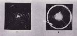
Plates 67a&b: Radio Interference
Click on Thumbnail to see Full-size image.
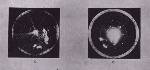
Plates 67c-d: Radio Interference
Click on Thumbnail to see Full-size image.
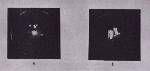
Plates 67e-f: Radio Interference
Click on Thumbnail to see Full-size image.
This type of interference
considerably reduces the effectiveness of the radar, but this type of
interference, taken alone, is usually readily identifiable by
operating personnel. This might not be as true when it occurs in
conjunction with extraordinary meteorological, propagation, and
equipment degradation phenomena.
this can still be a powerful signal, as it might have a sensitivity
of displaying signals as weak as from -50 to -80 db or less. It is
also likely that the out-of-band interference will be derived from
the nonlinear interaction of the desired return signal and the
out-of-band interfering signal. The resulting interaction (mixing) of
these signals in the receiver can generate still weaker
intermodulation products that fall within the passband of the system
circuits so that they are displayed. Spurious responses can occur at
other than the frequency to which the radar is tuned because of
inadequacies in the rejection of the unwanted frequencies in the
receiver. The inadequacy is caused by insufficient out-of-band filter
rejection coupled with a high level of RFI.
occasionally fail to function effectively. For all radar and other
electronic systems, an increasing amount of effort is expended to
reduce the occurrence of these degradations or failures and to
minimize their effects.
BACK To Table 1
Lobes and Reflections
Figure 11: Antenna Lobe Pattern
Click on Thumbnail to see Full-size image.
a single target can be shown as a collection of false targets. Such
target outputs from side lobe returns are generally systematically
located in the display relative to the main beam return signal.
Therefore, in general, side lobe return signals are readily
identifiable by the operator and will tend to cause obliteration of
other nearby target returns. Side lobe return signals usually bear a
fixed relationship of adjacent blips on an arc about each side of the
main target return. This is a common problem in ship radars where
another ship is being scanned broadside. The highly reflective ship
might have a return signal that will occur at the true range of the
ship, but will be contained in an arc exceeding 10°or 15°
instead of a single narrow blip.
both situations echoes were observed extending from the surface up to
70,000 ft. (the upper limit of the PPI scope). Before these vertical
protrusions to high altitudes were observed during anomalous
propagation conditions when the echoes were known to be from ground
clutter, it was not realized that they were from side lobes. As a
result, the side lobe echoes had not been recognized when measuring
thunderstorm heights and reported heights were much too great. On the
PHI side lobe, echoes took the form of narrow echo protrusions above
the location of strong targets. These protrusions were often
segmented due to nulls between side lobes, but in some cases were
continuous.
It changes its apparent distance and direction relative to the radar.
The double reflecting return echo is shown in the PPI display in the
direction at which the first reflecting surface is found. The echo
may, however, be displayed at a point at which there is no actual
target. Moving objects, such as automobiles or other objects capable
of reflecting electromagnetic waves may be obscured on the PPI by
ground clutter so they are not identified. It is obvious that ghost
echoes can show movement which is not possible with real vehicles.
Many unusual PPI observations have been explained in this manner.
Figure 12: Geometry of Reflection Echoes
Click on Thumbnail to see Full-size image.
at the same azimuthal bearing as the aircraft, while its range always
exceeds that of the aircraft. Consequently, on the PPI, the path of
this ghost always lies outside the aircraft path. However, if the
aircraft overflies the ground object, the phantom echo and the
aircraft echo will almost merge. In addition, as the apparent range
of the phantom is greater with the same radial speed as the aircraft,
the apparent velocity of the ghost will be magnified by the ratio of
the aircraft-to-phantom distance from the radar. The phantom can
appear to exceed 2,000 knots in this manner. In Fig. 13 the ghost is
moving at 900 knots along a portion of the ghost track.
Figure 13: Ghost Echo Track
Click on Thumbnail to see Full-size image.
Figure 14: Ghost Echo Track
Click on Thumbnail to see Full-size image.
it very difficult to discern whether the phantom was real or ghost.
He is concerned about the erratic behavior of a target, but he is
most concerned by the potential and displayed near-misses to known
targets.
as extraordinary meteorological conditions, and multiple-time-around
echoes can also be contributing effects, making the analysis that
much more difficult. When interference problems, operator
interpretation, and equipment reliability factors are included, one
begins to realize that the explanation of reported unusual
observations requires extensive research for each incident, and such
research is not possible unless all pertinent information has been
documented in detail.
BACK To Table 1
7. Evaluation of Radar Echoes to Identify Targets
Target Velocity
Target Intensity and Fluctuations
Behavior Relative To Other Targets
BACK To Section 7
Target Velocity
for 0.1 sec. as the beam sweeps past. Then 9.9 sec. elapse until the
beam again sweeps the target. If on this next revolution there is an
echo in the general vicinity of the target detected on the previous
sweep the operator must decide whether this echo is from the same
target that was detected previously or is from a new target. If he
assumes the two echoes are from the same target, he can then compute
a velocity. If his assumption was correct, if his computations are
accurate, and if the target is at the indicated locations, the
computed ground speed is correct. If, however, the two echoes are not
from the same target or are from a target that is not at the
indicated location, then the computed speed will have no meaning.
required for one antenna revolution. Such an assumption would
probably require a very high speed target. Or the operator might
assume that the target decreased altitude to a position below the
radar horizon. If the target was located close to the radar horizon,
an altitude change of a few tens of feet would be sufficient for it
to disappear and the required speed (vertical velocity) would be
quite small.
BACK To Section 7
Target Intensity and Fluctuations
of the signal intensity of targets at different ranges, so that the
operator loses much of the available radar information when it is
displayed on the PPI. Fluctuations are smoothed out, and the
intensities are normalized to some extent. The result is that he can
give some information on an unknown target in comparison with a known
target at the same range. Positive knowledge of the nature of
a target at a given range can only result from auxiliary data. For
example, if the operator is in contact with an aircraft that is over
a given point and he has an echo at that point he will logically
assume the echo is from the aircraft if the echo is moving on the
course and at the speed reported by the pilot. He could then compare
the intensity and fluctuations of other targets at that range with
those of the known target and draw some conclusions as to whether
they might be larger or smaller than the aircraft.
BACK To Section 7
Behavior Relative To Other Targets
of portions of the thunderstorms to the west. The obstacles causing
the reflections were subsequently identified as large nearby chimneys
that extended only slightly higher than the height of the radar so
that when the antenna was elevated slightly the chimneys were below
the main beam and no longer caused reflections.
of the true target toward or away from the reflector. This is not its
actual ground speed. A target could move at 500 knots along a
constant-distance circle from the reflector, yet the reflected echo
would be stationary. Only if the target moved directly toward or away
from the reflector would the reflected echo have the same speed as
the target; but the speed of the reflected echo can never exceed that
of the target.
The most complex cases are those in which a moving reflector is not
illuminating a single target but may show a different target on each
scan of the radar. In these cases there is no correspondence between
reflected echo track and reflector track. Speed computations in these
cases are erroneously based on multiple targets. Attempts to compute
a speed therefore produce values that can vary from some very low
speeds to thousands of knots.
BACK To Section 7
8. Conclusions
presentations show the interpreter apparent motion and
changes in intensity. This additional information is useful but still
does not permit positive identification of the target. Only such
generalizations may be made as that the target appears to be moving
at 250 knots so it cannot be precipitation, birds, or a balloon. To
even make this generalization the operator has to know or make some
assumptions about the probable wind speed in the vicinity of the
apparent target.
he will come to an erroneous conclusion.
Bibliography
Blackmer, R.H. Jr. and S.M. Serebreny. "Analysis of Maritime
Precipitation Using Radar Data and Satellite Cloud Photographs,"
J. Appl. Meteor., Vol. 7, (1968), 122-131.
Gunn, K.L.S. "Tube Space Filters for Line Space Compensations,"
Proc. Tenth Wx. Radar Conf., Wash., D.C., (1965).
Levine, D. Radargrammetry, McGraw Hill, N.Y. 1960.
Plank, V.G., R.M. Cunningham, and G.F. Campen, Jr. "The Refractive
Index Structure of a Cumulus Boundary and Implications Concerning
Radio Wave Reflection," Proc. Sixth Wx. Radar Conf. Cambridge,
Mass., (1957), 273-280.